 | 21 Aug 2019
2016 Central Italy Earthquakes: comparison between GPS signals and low-cost distributed MEMS arrays
Nicola Cenni
Filippo Casarin
Giancarlo De Marchi
Maria Rosa Valluzzi
Giorgio Cassiani
Modern seismic ground-motion sensors have reached an excellent performance quality in terms of dynamic range and bandwidth resolution. The weakest point in the recording of seismic events remains spatial sampling and spatial resolution, due to the limited number of installed sensors. A significant improvement in spatial resolution can be achieved by the use of non-conventional motion sensors, such as low-cost distributed sensors arrays or positioning systems, capable of increasing the density of classical seismic recording networks. In this perspective, we adopted micro-electro mechanical system (MEMS) sensors to integrate the use of standard accelerometers for moderate-to-strong seismic events. In addition, we analyse high-rate distributed positioning system data that also record soil motion. In this paper, we present data from the 2016 Central Italy earthquakes as recorded by a spatially dense prototype MEMS array installed in the proximity of the epicentral area, and we compare the results to the signal of local 1s GPS stations. We discuss advantages and limitations of this joint approach, reaching the conclusion that such low-cost sensors and the use of high rate GPS signal could be an effective choice for integrate the spatial density of stations providing strong-motion parameters.
- Article
(9855 KB) - Full-text XML
-
Supplement
(83 KB) - BibTeX
- EndNote


In 2016 an important seismic sequence took place in the Central sector of the Apennines belt, in the Italian peninsula (Fig. 1). The seismic sequence struck the region close to the towns of Norcia and Amatrice. The main shock events and the triggered aftershocks were located along the central part of the belt extending in NW-SE direction (Fig. 1). The first main shock with an estimated magnitude of Mw = 6 (Tinti et al., 2016), occurred at the 01:36:32 UTC of 24 August, with epicenter located near the towns of Accumoli and Amatrice (Fig. 1). The seismic sequence was characterized by numerous aftershocks. On 26 October an event of magnitude Mw = 5.9 (Tinti et al., 2016) shook again the central Apennines with an epicenter located northwest of the previous main earthquake. A stronger event occurred on 30 October at 06:40:17 UTC, with a magnitude of Mw = 6.5 (Tinti et al., 2016), with epicentre close to Norcia (Fig. 1). The fault plain solutions of these three main shocks (http://cnt.rm.ingv.it/tdmt, last access: 1 August 2019), exhibit normal faulting consistent with the tectonic regime of the area (Galadini et al., 2000). The Central Apennines are characterized by a Quaternary NE-SW oriented extensional regime (Boncio and Lavecchia, 2000; Mantovani et al., 2019). The kinematic pattern, inferred from the continuous GPS stations (e,g, Cenni et al., 2012), confirms that these extensional tectonic processes are still active. The horizontal GPS velocity field shows that the Eastern Adriatic sector of the Central Apennines moved significantly faster and more Easterly with respect the inner Tyrrehnian sector, with consequent development of extensional to transverse deformation in the axial part of the belt. The 2016 central Italy sequence was recorded by the Italian Seismic Network (RSN) and by the Accelerometers National Network (RAN). The main shocks of the sequence, and in particular the shocks of 24 August and 30 October, were also recorded by a prototype MEMS low-cost distributed array installed for research purposes (Boaga et al., 2018). Figure 2 shows the locations of the prototypal MEMS array, of the continuous GPS stations (CGPS) and of the Italian Seismic Network and Accelerometers Network stations in the area struck by the seismic events. The GPS sites shown in Fig. 2 are all equipped with a multi-frequency geodetic instruments and the observations, acquired with a 30 s sampling rate, have been used to estimate the co-seismic movements (e.g. Cheloni et al., 2016, 2017). Some authors (Avallone et al., 2016; Xiang et al., 2019) have also estimated the co-seismic dynamic displacements related to the 2016 main shocks analysing the observation acquired by the CGPS stations in the epicentral area with a higher sampling rate (≤1 s). A low-cost GPS network (equipped with single frequency instrument and they are not shown in Fig. 2) located near the epicenter of the 30 October event provides important information about the propagation of slip from depth on the surface rupturing (Wilkinson et al., 2017).
In this work, we compare the co-seismic displacements field as estimated by the high rate 1Hz daily position time series of the CGPS (located at a distance smaller than 100 km from the epicentres area) with the evidence collected by the prototype MEMS low-cost distributed array. We restricted ourselves to comparing the observation acquired by the closest MEMS and GPS stations located near Foligno (Fig. 1), in the relative far field of the seismic sequence, since some authors (e.g. Avallone et al., 2011) suggest that a 1 Hz–sampling GPS site located in the near source of a moderate magnitude event (M 6 class) can provides an aliased solution about the co-seismic time series.
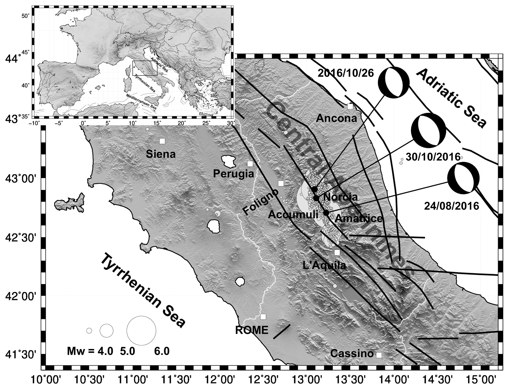
Figure 1The Central Italy earthquake sequence. The epicentres of the events occurring during the period 1 June 2016–26 December 2017, available from http://cnt.rm.ingv.it/ (last access: 1 August 2019), are indicated with the white circles, with size proportional to the moment magnitude (Mw). The thick black lines show the main tectonic lineaments from the Database of Individual Seismogenic Sources (DISS, Basili et al., 2008). The time domain moment tensor (TDMT) solutions of the three main shocks are also shown (INGV TDMT Catalog available at http://cnt.rm.ingv.it/tdmt, last access: 1 August 2019). Main cities and towns in the study area are shown with white squares. (Built with the Generic Mapping Tool software GMT – Creative Commons Attribution 4.0 License.)
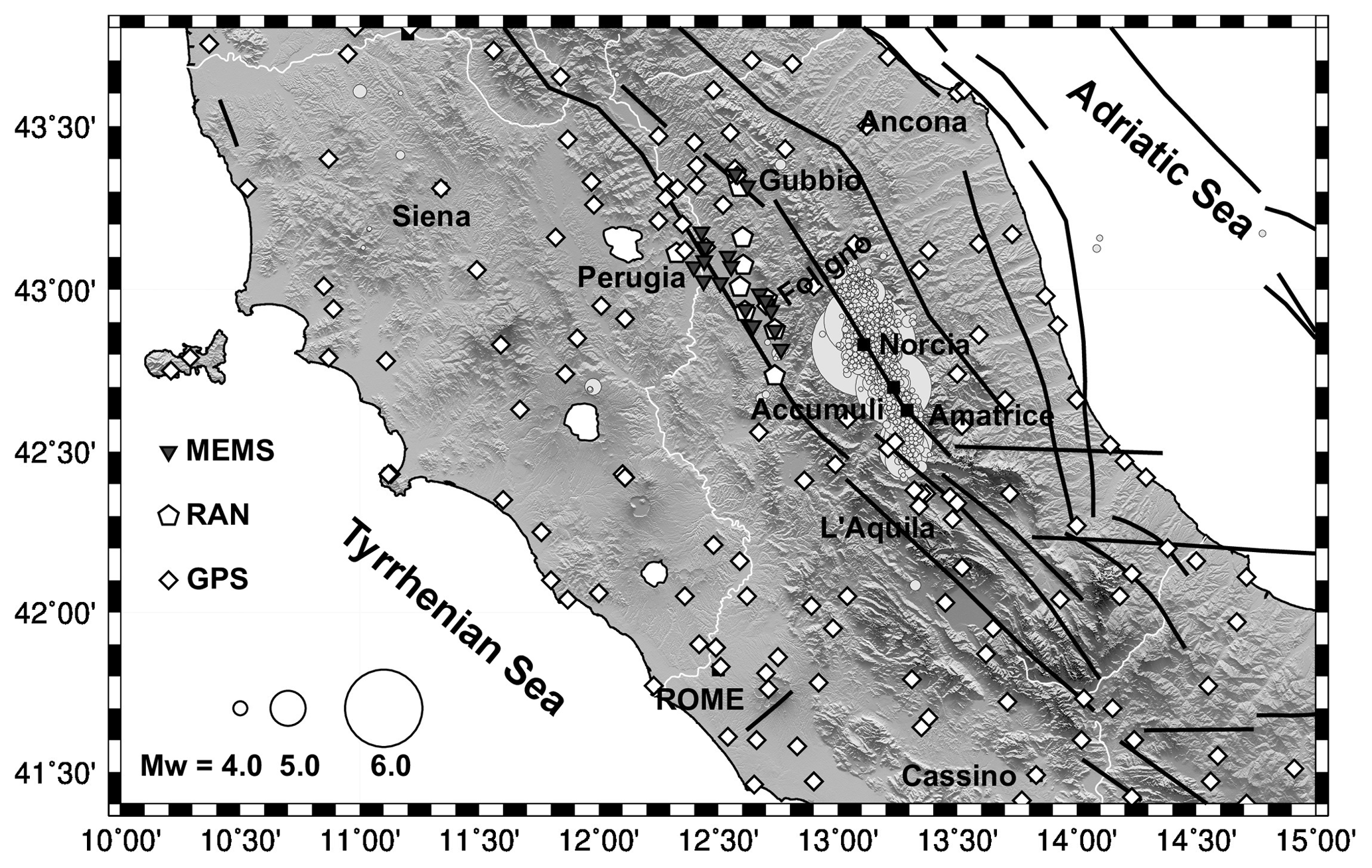
Figure 2MEMS, RAN and CGPS networks in the area impacted by the 2016 Central Italy earthquake sequence. The epicentres of the events occurring during the period 1 June 2016–26 December 2017 are shown as in Fig. 1. The diamonds and inverted triangles show respectively the locations of the continuous GPS stations and of the prototype MEMS low-cost distributed array. The white pentagons show the locations of the accelerometers of the National Network (RAN). The thick black lines are the principal tectonic lineaments from the Database of Individual Seismogenic Sources (DISS, Basili et al., 2008). (Built with the Generic Mapping Tool software GMT – Creative Commons Attribution 4.0 License.)
An efficient seismic wavefield recording is achieved if the network has sufficient sensors dynamic range, frequency response and spatial resolution (Evans et al., 2005). The first two aspects can be tackled by the installation of modern seismographs with very large dynamic range (> 120 dB) and broadband response (10−2 to 102 Hz). The weak point in the experimental seismic response analysis still remains the limited number of sensors installed throughout the territory. Densely distributed arrays would lead to better earthquake localization and local seismic response definition, but the use of high-quality sensors makes this option prohibitively expensive, in terms of both purchase and maintenance costs. An alternative approach can be based on the use of cheaper sensors such as Micro Electro-Mechanical Systems sensors known as MEMS (Fleming et al., 2009; Evans et al., 2014). Analogic and digital MEMS technology has proven to reach a performance efficient enough to be adopted as ground motion accelerometers for moderate (M > 4) to strong seismic events (D'Alessandro et al., 2014; Lawrence et al., 2014; Boaga et al., 2019). Nowadays, MEMS can easily meet the moderate-to-strong motion seismological needs, having instrumental noise of ≈100 µg Hz, a fairly broad frequency response and an acceleration range up to 1–4 g.
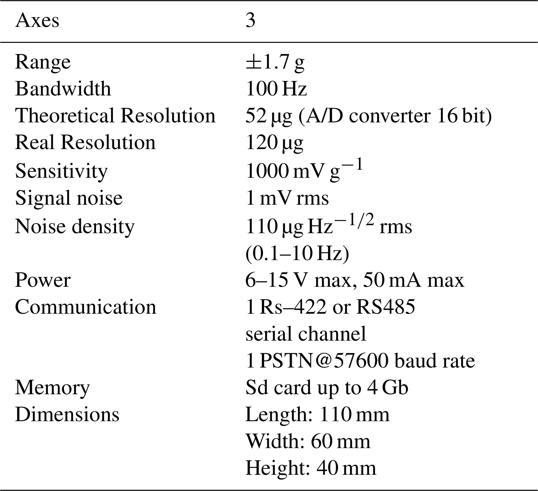
In the spring of 2016 we installed 20 prototypes of MEMS accelerometers in the Perugia – Foligno area in the Central Apennines (Fig. 2). The MEMS network was installed in the local telecommunication infrastructures (owned by Telecom Italia Mobile – TIM S.p.A.), originally for infrastructure monitoring purposes. The MEMS accelerometers are new prototypes designed and built by AD.EL, a company specialised in distributed sensors and telecommunication supplies. The MEMS prototypes, named D600003A, were first tested under excitations at sweeping frequencies in a certified shaking table, giving deviation compared to the reference of less than 0.3 % for frequencies below 20 Hz in the acceleration range 0.1–10 m s−2. The MEMS sensor has small size () and includes: 3 component accelerometers, a local storage card and several possible communications options from cable Ethernet transmission to GPRS communication tool. Timing was provided by an external GPS antenna. The technical specifications of D600003A are provided in Table 1.
Table 1Technical specifications of the ADEL D600003A MEMS accelerometer.
The prototype MEMS sensor arrays recorded the main shocks of 24 August and 30 October of the Central-Italy 2016 sequence. The resulting data are of good quality, especially if compared to the closest high-quality National Accelerometers Network stations (RAN see Fig. 2) – see Boaga et al. (2018) for details. The National Accelerometers Network stations (RAN, ran.protezionecivile.it) adopt conventional high quality strong motion sensor such as the Kinemetrics Episensor ES-T (kinemetrics.com/post_products/episensor-es-t). Figure 3 shows, as an example, the comparison between MEMS and the high-quality RAN station close to the city of Gubbio and Spello for the 2 main earthquakes of 24 August and 30 October. The stations inter-distances were less than 0.2 km and both are located in the same soil condition. Both peak ground acceleration and spectral response are comparable, especially in the range of interest for a-seismic design (0–15 Hz).
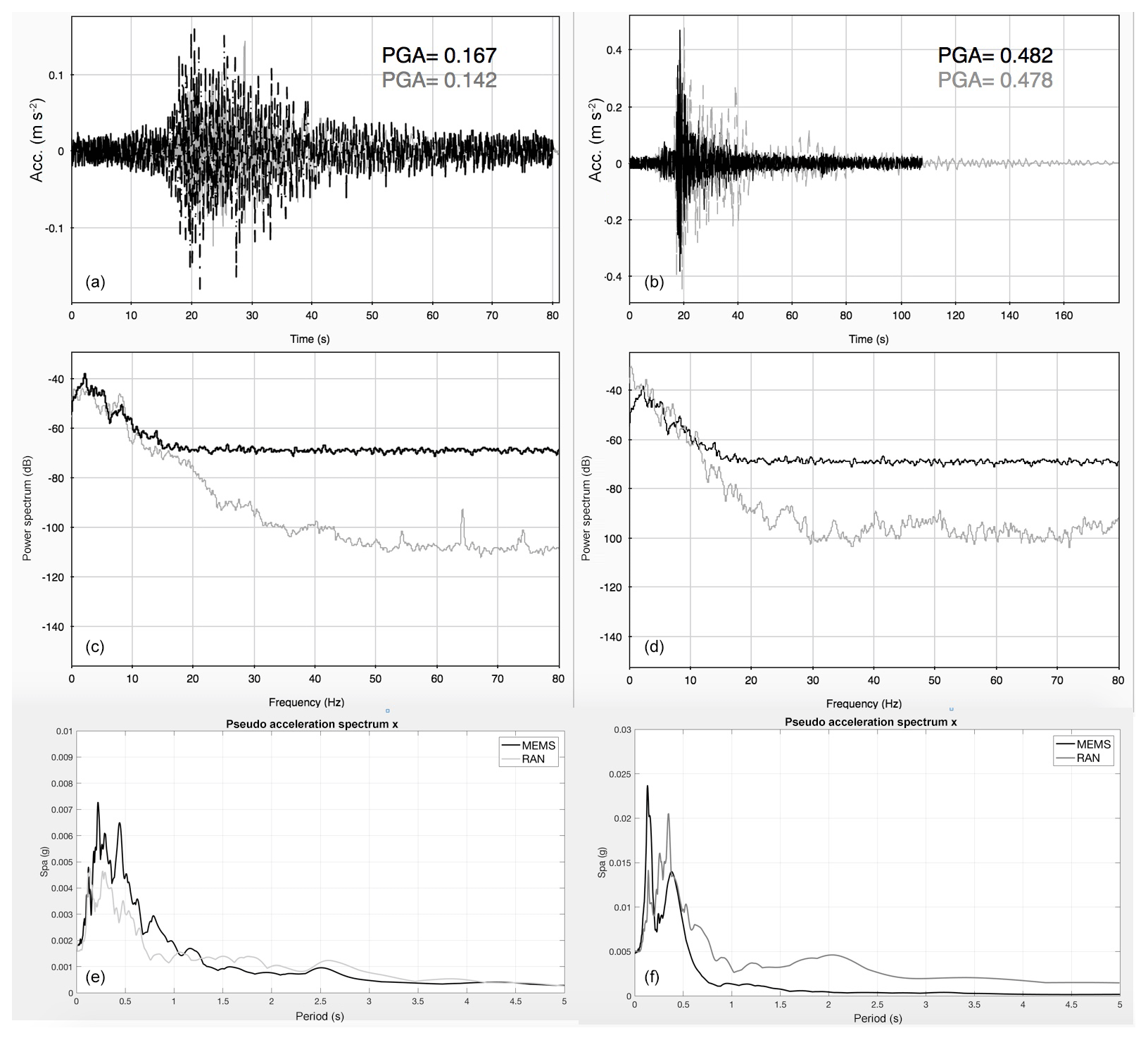
Figure 3Comparison between MEMS based prototypes (black) and closest RAN sensors (grey) for the 24 August “Accumoli” earthquake (a, c, e) and the 30 October “Norcia” earthquake (b, d, f). (a, b) “Spello” and “Padule” MEMS time series are compared to national stations RAN “CSA” and “GBC”; (c, d) frequency domain responses; (e, f) Elastic response spectra in the period range 0–5 s (5 % damping).
The earthquake sequence occurred in an area where a number of scientific and technical continuous GPS (CGPS) stations are active (Fig. 2). An accurate study of the CGPS time series can provide information about co-seismic and post seismic displacements, as proven by many authors (e.g. Cheloni et al., 2017; Cenni et al., 2012; Savage and Langbein, 2008).
The GPS observations, acquired with a sampling rate of 30s, were initially analysed using the GAMIT/GLOBK software, 10.7 release (Herring et al., 2018a, b) adopting a distributed approach (Dong et al., 1998; Cenni et al., 2012, 2013). This procedure provides the daily time series of the local geodetic components North, East and Vertical for each position, referred to the international frame ITRF2014 (Altamimi et al., 2016). The estimated time series were then analysed separately by the procedure suggested by Cenni et al. (2012, 2013) in order to estimate: (i) the tectonic velocity, (ii) the discontinuities due to seismic events and instrumental features, (iii) seasonal signals and noise. The daily positions were firstly processed to detect and remove outliers, allowing a preliminary estimation of velocity and displacement values. A theoretical model of the time series is then estimated and subtracted from the observed data. The residual time series are then analysed adopting the Lomb (1976) and Scargle (1982) approach in order to evaluate the first 5 frequencies with the most powerful peaks in the interval between one month and half of the observation time span. These frequencies have been successively considered for a more detailed model of the coordinate time series:
where k is the local geodetic component of the position (North = 1, East = 2 and Vertical = 3), Ak and vk are the intercept and tectonic velocities, is the amplitude of the l seasonal signal with period Pl, gkj terms are the estimated offset magnitudes for the N discontinuities due to instrumental changes or seismic events eventually occurred at the Tj epochs, while H is the Heaviside step function, εk (ti) is the error term.
The parameters can be estimate by the Weight Least Squared Method (WLSM), highlighting the discontinuities due to events or instrumental changes which occurred in a time span of few days. The lack of data between two discontinuities can limit the reliability the displacements estimation. This problem could manifest itself when two or more seismic events occur in a few days, as for example in the central Italy sequence where the main event of the 30 October (Mw = 6.5) occurred only 4 d after another shock of Mw = 5.9. During these few days the operations of several CGPS sites could have been interrupted and the observations lost. For these reasons, here we focus on the 24 August earthquake main shock data, in order to use all available stations data. The geodetic displacements for the 24 August earthquake are shown in Fig. 4. The estimated co-sesmic displacements are also reported in Table A1 (Appendix A1).
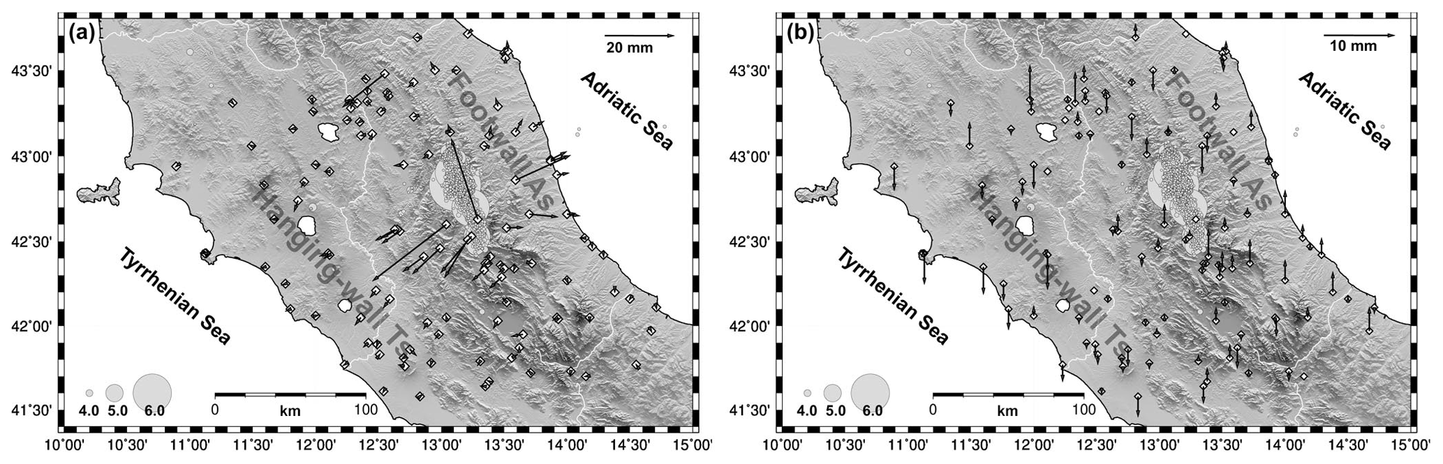
Figure 4Horizontal (a) and Vertical (b) co-seismic displacements due to the 24 August 2016 main event. The displacements (millimetres) are estimated analysing the coordinate time series of the continuous GPS permanent stations located at a distance smaller than 100 km from the epicentral area. The white diamonds indicate the locations of the CGPS sites. The epicentres of the events occurring during the period 1 June 2016–26 December 2017 are also reported in the Figure, with the circles' size of proportional to the moment magnitude. Ts = hanging-wall Tyrrhenian sector; As = footwall Adriatic sector. (Built with the Generic Mapping Tool software GMT – Creative Commons Attribution 4.0 License.)
The co-seismic patterns shown in Fig. 4 are consistent with the activation of a SW dipping normal fault system and the results obtained by other research groups (e.g. Cheloni et al., 2016, 2017). The horizontal field is characterized by a general SW-NE oriented extension, while the vertical movements show a more heterogeneous pattern. In particular, the stations located within few tens of km from the epicentre and placed on the hanging-wall Tyrrhenian sector (Fig. 4) present an uplift not completely coherent with a normal fault source as described by the focal mechanism. The recorded displacements are anyway in good agreement with InSAR observations analysed by Bonini et al. (2016). The vertical field on the footwall Adriatic sector (Fig. 4) shows a more coherent pattern, even if some sites located at few tens of km from the event show a non-negligible subsidence in contrast with the movements of the entire structure. These differences could be due to local movements of the building where the CGPS stations are installed, or to local displacements.
Over the past decade, several authors (Avallone et al., 2009, 2012; Bock et al., 2004; Cheloni et al., 2016; Wang et al., 2007; Xiang et al., 2019) demonstrated that the GPS instruments are able to infer the dynamic features of fault rupture processes, when they are set up with an high frequency sampling interval (≤1 Hz). These dynamic observations are several orders of magnitude less sensitive than the common high quality seismometers readings, but do not suffer from drift, clipping, or instrument tilting (Avallone et al., 2009). The so-called High-Rate GPS (HRGPS) time series have been recently compared with the strong motion data acquired from high-quality accelerometric networks (Cheloni et al., 2016). In this work we want to compare the HRGPS series with the data acquired from the low-cost MEMS prototype distributed network, in order to understand if such not-conventional networks can be also adopted to retrieve seismic motion parameters. We used the available high rate recordings of the CGPS stations compared to the closest available MEMS data (see Table 2). We selected the area close to Foligno (Fig. 5) that hosts a CGPS station, with observations acquired during the events with a sampling rate of 1 Hz, and 4 MEMS sensors in the surrounding (named respectively B00393, B00396, B00399 and B00402).
Table 2Distances in km between the MEMS accelerometers and the Foligno CGPS site (FOL1, Fig. 5), and the earthquake epicentre of 24 August 2016 event. The North and East columns contain the distance along these horizontal components, while in the Dist. columns we report the modulus of the horizontal distance.
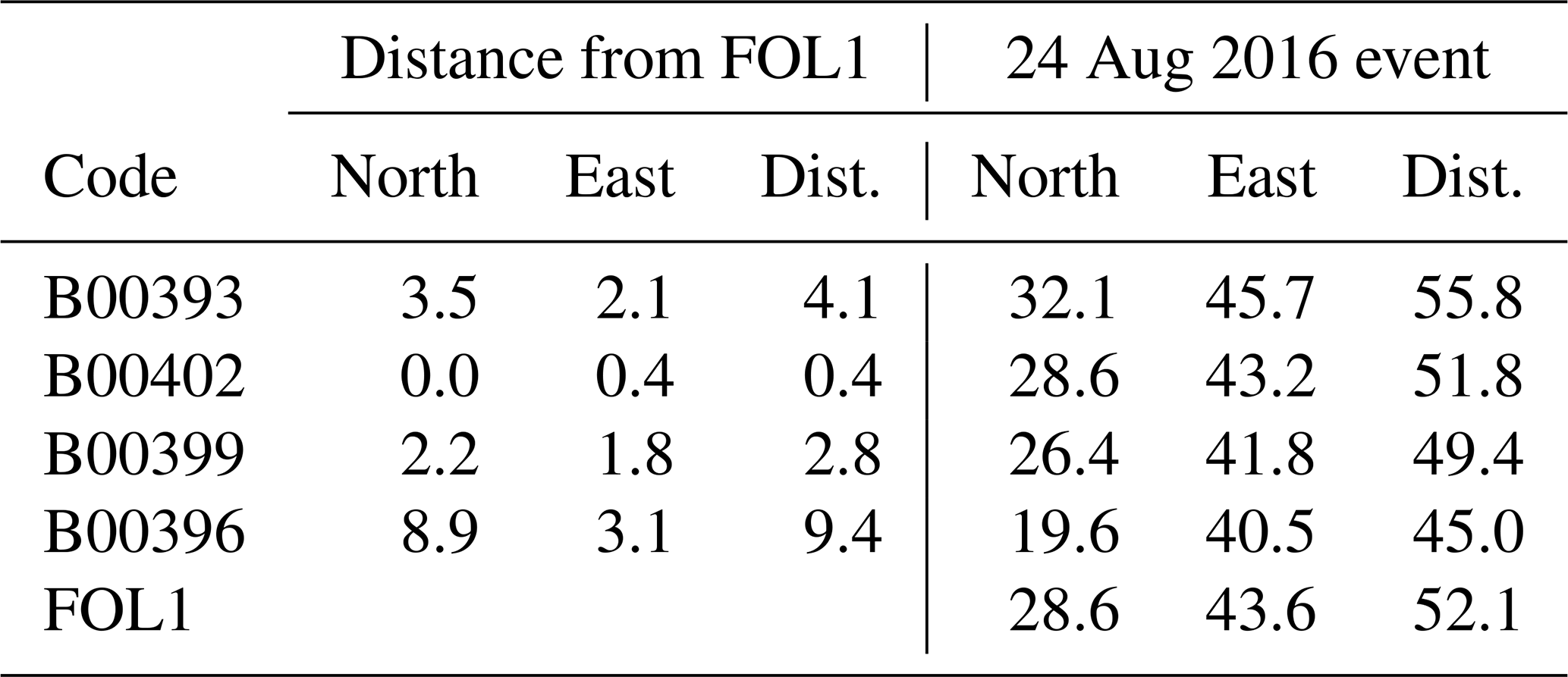
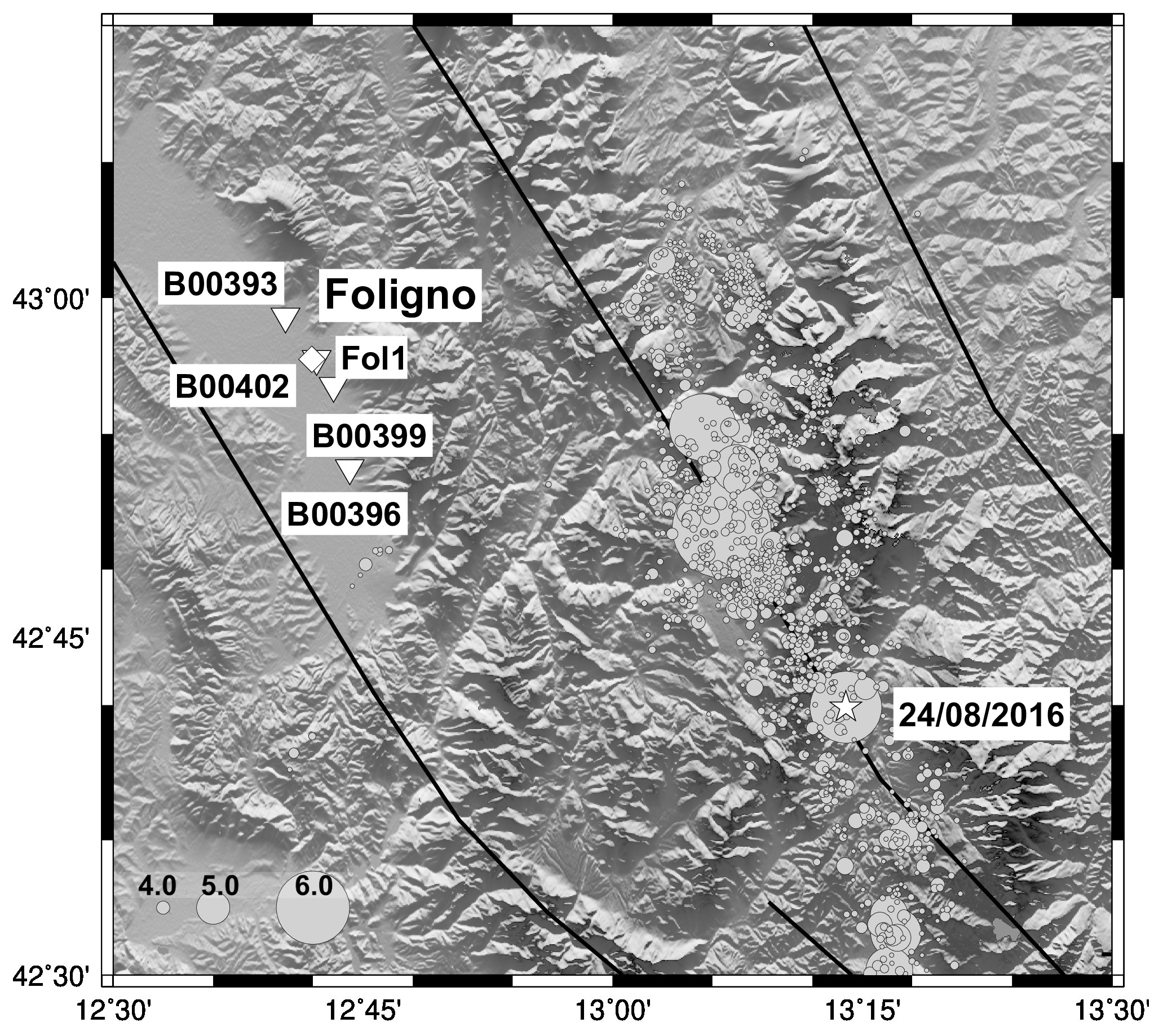
Figure 5Location of the Foligno CGPS site (FOL1, diamond) equipped with a sampling rate of 1 Hz and the closest (distance < 10 km) MEMS sensors in the area (inverted triangle). The thick back lines show the principal tectonic lineaments from the DISS database of Individual Seismogenic Sources (DISS, Basili et al., 2008). The epicenters of the events occurring during the period 1 June 2016–26 December 2017 are indicated with gray circles, the size of the symbols are proportionally to the moment magnitude (Mw) following the scale on the figure. The star indicates the location of the 24 August 2016 main shock. (Built with the Generic Mapping Tool software GMT – Creative Commons Attribution 4.0 License.)
The GPS observations at 1 Hz sampling have been analysed using the GAMIT/GLOBK software (Herring et al., 2018a, b), using the kinematic module TRACK. This module performs a relative kinematic positioning, where it is necessary to define a reference station. The reference observations should be not affected to the dynamic displacement due to the seismic rupture. Therefore, we assumed as a reference station the Cassino site (CASS, Figs. 1 and 2), that is located outside the strike area of the earthquake. The distances between the GPS station and the MEMS sensors are smaller than 10 km, and two accelerometers are particularly close to the Foligno CGPS station with distance within 1.5 km range. In order to get a fair comparison between data, the MEMS observations have been decimated at the same frequency (1Hz) of the GPS data.
The noise level in the time series must be taken into account in order to investigate whether dynamic displacements due to the seismic event can be detected by the HRGPS station. As a representative level of the noise we have taken the Root Mean Square (RMS) value estimated during the time interval ranging from 90 s before the origin time of the event (01:36:32 UTC, Marchetti et al., 2016) and 10 s afterwards (we considered the data up to 10 s after the UTC main shock because the MEMS and HRGPS Foligno arrays are located about 50 km from the epicentral area, so not including the event). The estimated RMS values of the HRGPS components and MEMS time series are reported in Table 3.
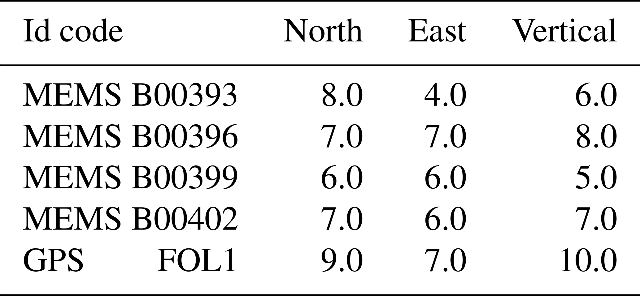
Table 3Root Mean Square (RMS) values of the HRGPS and MEMS time series estimated using the data available from 90 s before and 10 s after the main UTC time of the event, during quite acquisition time. The GPS and MEMS values are respectively in mm and m s−2. The columns reported the values estimated analysing the time series of the North, East and Vertical components.
4.1 Results
Figure 6 shows the HRGPS displacement time series and the MEMS accelerations acquired during the 24 August earthquake. The horizontal axis in Fig. 6 is scaled in seconds from the main shock origin time (01:36:32 UTC, Marchetti et al., 2016). The North component of Fol1 GPS station (thick dashed line in Fig. 6) shows an initial displacement of about 30 mm peak-to-peak, while the displacement along the East coordinate is about 20 mm peak-to-peak. These values are about twice the RMS values reported in Table 3, assumed as the noise amplitude of the time series. The co-seismic dynamic displacements observed on the vertical component are conversely similar to the RMS value (about 10 mm), therefore it is difficult to identify the first arrival of the seismic sequence and the other seismic signals. The inelastic co-seismic movements observed at the same station are shown in Fig. 4 and are of −3.4 and −0.6 mm (Table A1) along respectively the East-West and North-South directions, while the vertical component shows a subsidence of −2.1 mm (Table A1). These values are one order of magnitude lower than the initial elastic displacements observed in the HRGPS time series during the event.
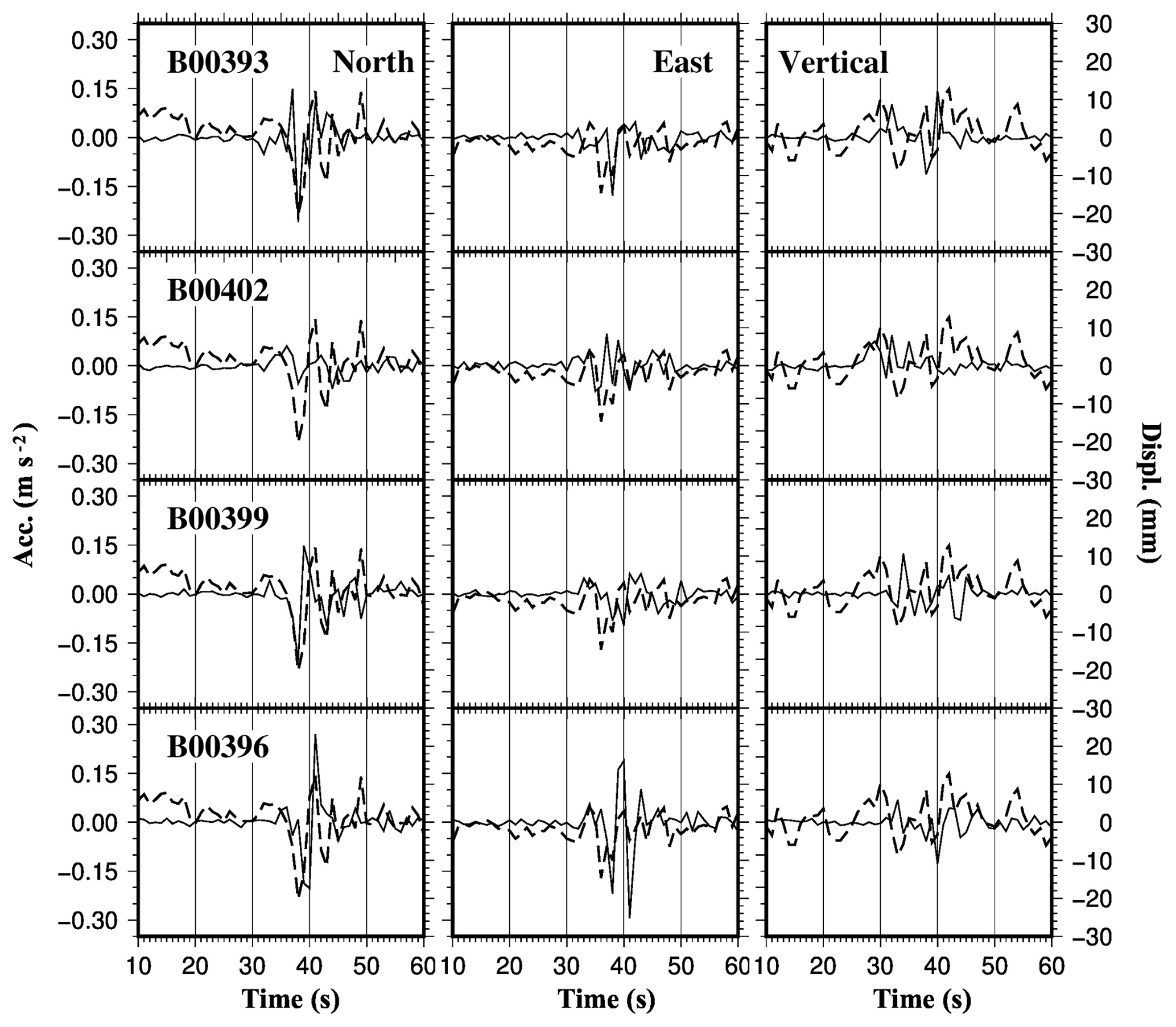
Figure 6GPS-derived displacement waveform recorded at the Foligno permanent station (thick dashed line) and low-cost MEMS array signals (thin solid line). Observations are presented for the three local geodetic components: North, East and Vertical, with the same sampling rate of 1 Hz. The MEMS instrument code is reported in each figure. The horizontal axis is given in seconds after the main shock origin time: 01:36:32 UTC of 24 August 2016. The right vertical axis denotes GPS displacements, while accelerations refer to the left axis. According to the epicentral distances, the MEMS signals of the four stations are arranged in decreasing order from top to bottom. (Built with the Generic Mapping Tool software GMT – Creative Commons Attribution 4.0 License.)
The local geodetic coordinate system adopted to show the results in Fig. 6 is probably non optimal to compare the high rate GPS time series against the data from MEMS. Therefore, the horizontal components (North and East) of GPS and MEMS sensors have been rotated with respect to the epicenter and presented in the Radial-Transverse (RT) coordinate system. The azimuth angle adopted to rotate the horizontal components in the RT system is 303∘ as suggested to other authors (Avallone et al., 2016). The radial component should contain mainly P and SV-wave arrivals, while the SH-wave modes should be predominant in the transverse component.
To analyse the similarity between MEMS and HRGPS observation we have transformed in displacements the MEMS recording by applying a double-integration. We have firstly filtered the MEMS and HRGPS observations by a Butterworth high pass filter. Figures 8 and 9 show respectively the MEMS and HRGPS displacements times series of the local geodetic components (North, East, Vertical) and the ones in the RT coordinate system.
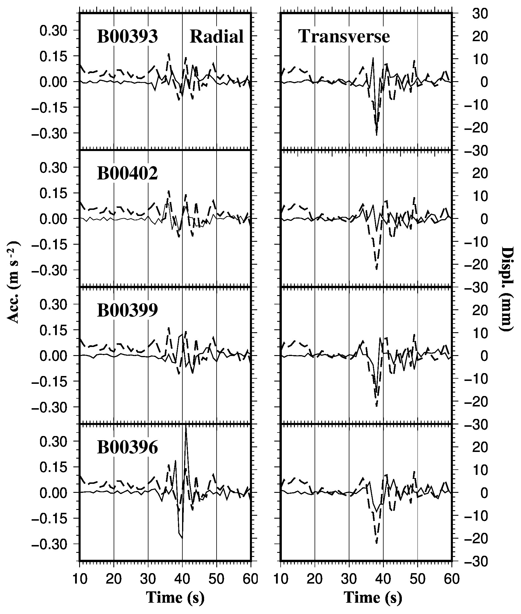
Figure 7Acceleration time series from MEMS and HRGPS displacements in the Radial-Transverse coordinate system. The thick dashed lines represent displacement estimated using the HRGPS displacements of the Foligno (FOL1) permanent site. The thin solid lines show acceleration time series recorded at four different MEMS stations – the code of each instrument is reported. The MEMS signals of the four stations are arranged in decreasing order from top to bottom according to epicentral distances. The horizontal axis denotes seconds from the origin time of the main shock: 01:36:32 UTC of 24 August 2016. The right vertical axis denotes GPS displacements, while accelerations refer to the left axis. (Built with the Generic Mapping Tool software GMT – Creative Commons Attribution 4.0 License.)
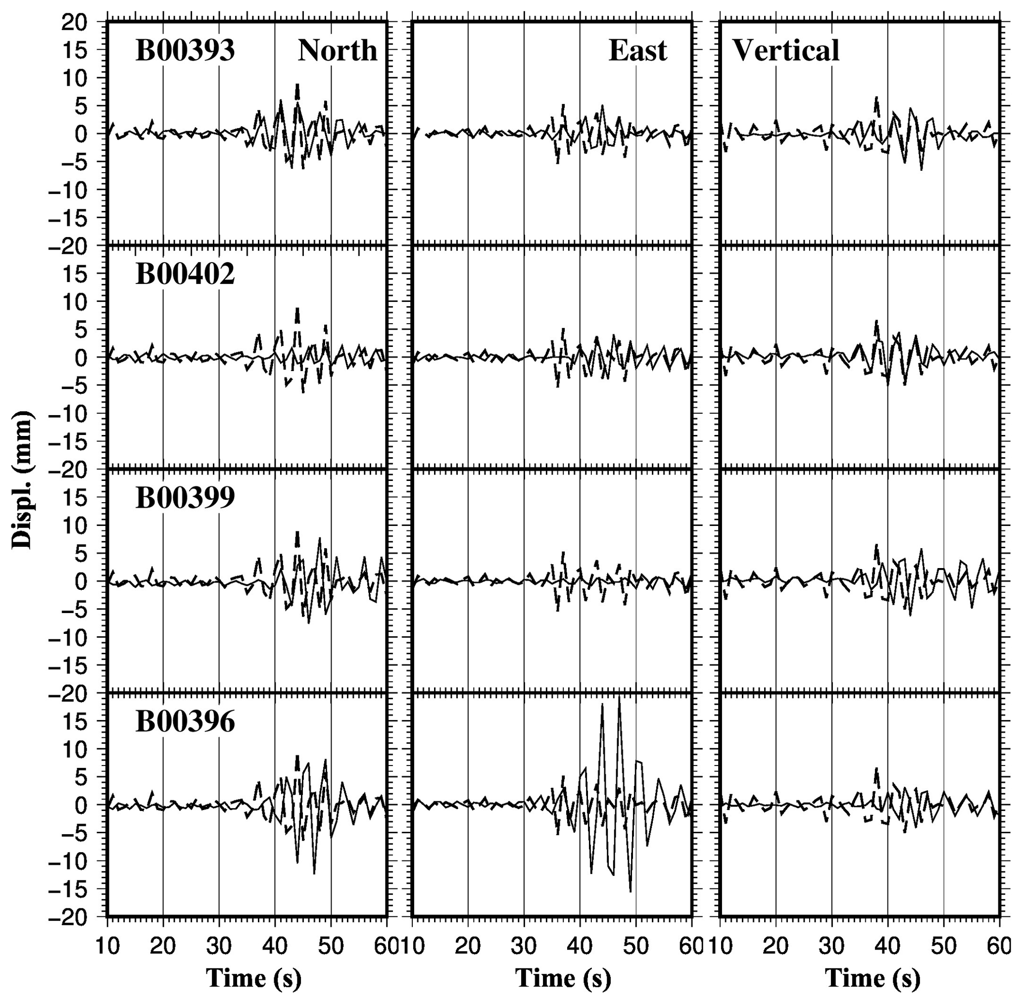
Figure 8MEMS (thin solid line) and HRGPS (thick dashed line) displacements time series obtained after the filtering and the double-integration. Observations are presented for the three local geodetic components: North, East and Vertical, with the same sampling rate of 1 Hz. The MEMS instrument code is reported in each figure. The horizontal axis is given in seconds after the main shock origin time: 01:36:32 UTC of 24 August 2016. According to the epicentral distances, the MEMS signals of the four stations are arranged in decreasing order from top to bottom. (Built with the Generic Mapping Tool software GMT – Creative Commons Attribution 4.0 License.)
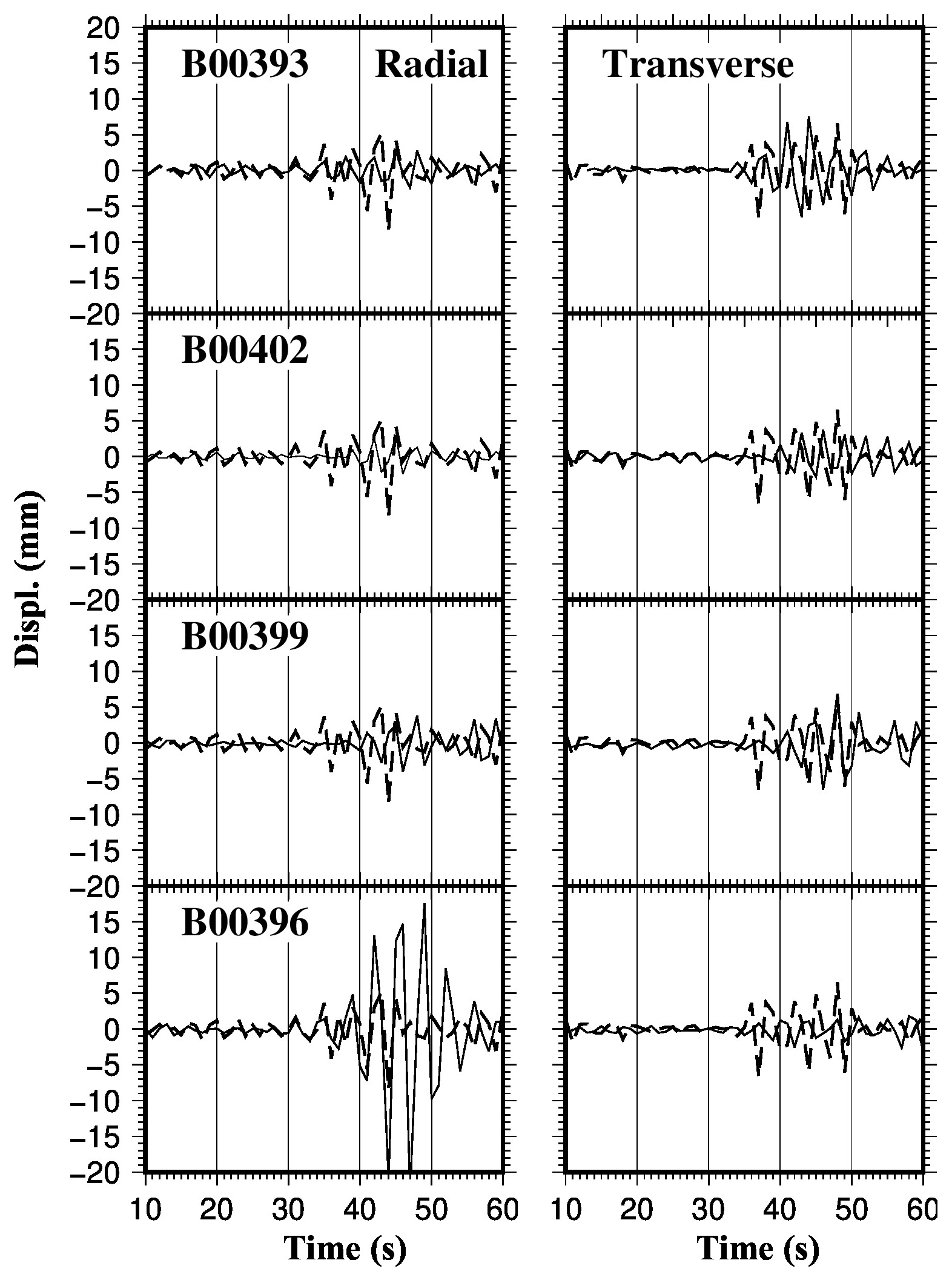
Figure 9MEMS and HRGPS (thick dashed line) displacements in the Radial-Transverse coordinate system. Thick dashed lines and thin solid lines represent respectively the HRGPS and MEMS displacements. The MEMS signals of the four stations are arranged in decreasing order from top to bottom according to epicentral distances, and the code of each instrument is reported on the figures. The horizontal axis denotes seconds from the origin time of the main shock: 01:36:32 UTC of 24 August 2016. (Built with the Generic Mapping Tool software GMT – Creative Commons Attribution 4.0 License.)
The displacement waveforms of the MEMS network and GPS station are qualitatively in agreement (Figs. 8 and 9). The displacement amplitude observed by the MEMS instruments are in fact similar to ones registered on GPS sites. Only the B00396 MEMS radial component presents greater displacement compared to the HRGPS station ant others MEMS stations. These differences are probably due to the large distance between the B00396 and GPS (about 9 km, Table 2) and the other accelerometers (Table 2). Also, the B00396 site is the closest to the earthquake respect the other MEMS and the FOL1 station. It can be noted as the displacements observed by MEMS and GPS at greater distance from the epicenter (about 50–55 km, Table 2) present similar displacement values (Figs. 8 and 9).
In order to quantify the similarity between the MEMS and GPS displacements we have estimated the correlation coefficients between the time series (Table 4). In particular, we have estimated the values analysing the displacements observed in the 30–40 s period after to the main shock event (01:36:32 UTC). It can be noted in fact in Figs. 8 and 9 as the first arrivals in the time series appears about 30 s after the main shock origin time.
Table 4Absolute Correlation coefficients estimated comparing the double-integrated MEMS data and GPS displacements filtered time series. The values refer to the time interval between 30 and 40 s after the origin time of the main shock (01:36:32 UTC).
The average absolute values of the correlation coefficients is 0.5, if we consider the 30–40 s period after the main shock in radial and transverse components (Fig. 9). This indicates a quite agreement between the waveforms compared, in particular between the components of the CGPS station and the MEMS sensors located at a relative distance lower than 3 km (Table 2). The worst values are observed in the comparison between FOL1 GPS station and the B00393 MEMS site, probably due to the relatively weak signals observed in this MEMS site (Figs. 8 and 9). B00393 is located at a distance of about 56 Km from the epicenter (Table 2), and the noise in the time series could be comparable with the amplitude of the seismic signals.
We compared the seismic motion during the 2016 Central Italy Earthquakes as recorded by two types of non-conventional sensors arrays: a distributed low-cost MEMS network and the local continuous GPS stations. Even if both network are initially designed for different purposes, the motion results are comparable (Figs. 8 and 9) and potentially useful to integrate the data recorded by the conventional high-quality seismic motion network. The low-cost distributed MEMS network was initially installed for telecommunication infrastructures monitoring but, for such moderate events as the 2016 Central Italy sequence, proved to be comparable in terms of motion response to high-quality sensors (Boaga et al., 2019). On the other hands the CGPS stations have been adopted for decades to evaluate tectonic patterns and relative displacements, but only recently the High-Rate GPS (HRGPS) time series proved to be sensitive to real–time seismic motion in case of moderate-strong earthquakes (eg. Avallone et al., 2016, 2012; Larson et al., 2003; Larson, 2009; Miyazaki et al., 2004; Xiang et al., 2019). We compared the displacements estimated by the accelerograms recorded by the low-cost MEMS instruments and the displacements observed from the closest High-Rate GPS station for the main shock of the 2016 central Italy sequence, i.e. the Mw = 6 event occurred on 24 August at 01:36:32 UTC. The time series analysed coming from these two non-conventional sensor arrays present promising similarity, especially for the horizontal components of motion (Fig. 9). In particular the quite agreement in the radial and transverse components between the GPS and MEMS located at a distance lower than 3 km (Fig. 9 and Table 4).
In particular, the MEMS and GPS displacement waveforms registered few seconds after the first arrival show interesting similarity: the displacements observed from the two instruments are of few millimetres, while absolute value of correlation coefficients of the main event indicate a quite agreement between the waveforms (Table 4). The differences in the second part of the seismograms are probably due to the different characteristics of the instruments and the sites where they have been installed.
The Foligno continuous GPS station has been installed and managed for professional positioning purposes, therefore not for scientific monitoring of the central Apennines area. The GPS antennas in such technical sites are usually installed on a steel bar anchored to the roof of a building or iron/steel pipes solidly connected to supporting walls. This non-geophysical installation could introduce different amplifications of the horizontal and/or vertical components as a response to the co-seismic shacking of the building. Also, the MEMS and GPS instruments are not located in the same position (the minimum distance is about 400 m, Table 2), therefore local site effects could introduce some differences in the seismic response of the sites and in the time series observed.
This study confirms that the GPS observations can detect both the co-seismic static displacements and the body-wave-arrival dynamic displacements. However, the quite agreement between the GPS and MEMS waveforms suggest the possibility to augment a seismic network with such a not-conventional arrays, in order to provide important information about earthquake radiation pattern, source parameters and site effects. In particular, the low cost MEMS distributed array and CGPS sampled at high rate would provide helpful contributions in case of moderate to strong-motion events.
GNSS DATA are available at “High-Rate GPS data archive of the 2016 Central Italy seismic sequence” Ring-INGV repository (ftp://gpsfree.gm.ingv.it/amatrice2016/hrgps/data/, last access: 1 August 2019). MEMS data are property of the company owner of the prototype network and are not public available. Private request can be sent to AD.EL srl, Martellago, Venezia , Italy.
The supplement related to this article is available online at: https://doi.org/10.5194/adgeo-51-1-2019-supplement.
Table A1Coseismic displacements determined for the GPS stations lying within 100 km from the epicenter of the 24 August main shock. The GPS code of the CGPS site is reported on the first column, the geographical coordinate (Lon = Longitude and Lat = Latitude) are reported in the second and third column. Dn, De and Dv are respectively the coseismic anelastic displacement along the North, East and Vertical direction. The uncertainties associated to the coseismic displacements have been estimated by a Weight Least Square Method adopted to evaluate velocity, discontinuities due to earthquakes and/or equipment changing and seasonal signals, as discussed briefly in the text (Cenni et al., 2012, 2013).
NC extracted and processed the GNSS data. He has also collaborated to comparison between the series. JB, FC and MRV processed the MEMS data. GdM furnished the MEMS prototype characteristics and data. GC evaluated the comparison and wrote the manuscript.
The authors declare that they have no conflict of interest.
This article is part of the special issue “Improving seismic networks performances: from site selection to data integration (EGU2019 SM5.2 session)”. It is a result of the EGU General Assembly 2019, Vienna, Austria, 7–12 April 2019.
We thank the Editor Damiano Pesaresi, Sebastiano Trevisani and an anonymous reviewer for constructive observations. Authors wish also to thank “TIM spa” for the authorization to the use of their telecommunication infrastructure during the installation of the prototypal MEMS arrays. Authors thank AD.EL srl for the use of MEMS proprietary data. We thank also all public and private institutions that manage and distribute the GPS data used in this work, and in particular: DPC (Dipartimento Protezione Civile, Italy), EUREF, ISPRA (Istituto Superiore per la Protezione e la Ricerca Ambientale, Italy), Italian Space Agency (ASI), Leica Geosystem for the ItaPos network, GeoTop srl for the NetGeo network, Regione Abruzzo, Regione Lazio and Regione Umbria.
This paper was edited by Damiano Pesaresi and reviewed by two anonymous referees.
Altamimi, Z., Rebischung, P., Métivier, L., and Collilieux, X.: ITRF2014: A new release of the International Terrestrial Reference Frame modeling nonlinear station motions, J. Geophys. Res.-Sol. Ea., 121, 6109–6131, https://doi.org/10.1002/2016JB013098, 2014.
Avallone, A., Marzario, M., Cirella, A., Piatanesi, A., Rovelli, A., Di Alessandro, C., D'Anastasio, E., D'Agostino, N., Giuliani, R., and Mattone, M.: Very high rate (10 Hz) GPS seismology for moderate-magnitude earthquakes: The case of the Mw 6.3 L'Aquila (central Italy) event, J. Geophys. Res.-Sol. Ea., 116, 1–14, https://doi.org/10.1029/2010JB007834, 2011.
Avallone, A., Latorre, D., Serpelloni, E., Cavaliere, A., Herrero, A., Cecere, G., D'Agostino, N., D'Ambrosio, C., Devoti, R., Giuliani, R., Mattone, M., Calcaterra, S., Gambino, P., Abruzzese, L., Cardinale, V., Castagnozzi, A., De Luca, G., Falco, L., Massucci, A., Memmolo, A., Migliari, F., Minichello, F., Moschillo, R., Zarrilli, L., and Selvaggi, G.: Coseismic displacement waveforms for the 2016 August 24 Mw 6.0 Amatrice earthquake (central Italy) carried out from high-rate GPS data, Ann. Geophys., 59, 1–11, https://doi.org/10.4401/ag-7275, 2016.
Basili, R., Valensise, G., Vannoli, P., Burrato, P., Fracassi, U., Mariano, S., Tiberti M. M., and Boschi, E.: The Database of Individual Seismogenic Sources (DISS), version 3: Summarizing 20 years of research on Italy's earthquake geology, Tectonophysics, 453, 20–43, https://doi.org/10.1016/j.tecto.2007.04.014, 2008.
Boaga, J., Casarin, F., De Marchi, G., Valluzzi, M. R., Cassiani, G.: Central Italy Earthquakes Recorded by Low Cost MEMS Distributed Arrays, Seismol. Res. Lett., 90, 672–682, https://doi.org/10.1785/0220180198, 2018.
Bock, Y., Prawirodirdjo, L., and Melbourne T.I.: Detection of arbitrarily large dynamic ground motions with a dense high-rate GPS network, Geophys. Res. Lett., 31, L06604, https://doi.org/10.1029/2003GL019150, 2004.
Boncio, P. and Lavecchia, G.: A structural model for active extension in Central Italy, J. Geodyn., 29, 233–244, https://doi.org/10.1016/S0264-3707(99)00050-2, 2000.
Bonini, L., Maesano, F. E., Basili, R., Burrato, P., Carafa, M. C. M., Fracassi, U., Kastelic, V., Tarabusi, G., Tiberti, M. M., Vannoli, P., Valensise, G.: Imaging the tectonic framework of the 24 August 2016, Amatrice (central Italy) earthquake sequence: New roles for old players?, Ann. Geophys., 59, https://doi.org/10.4401/ag-7229, 2016.
Cenni, N., Mantovani, E., Baldi, P., and Viti, M.: Present kinematics of Central and Northern Italy from continuous GPS measurements, J. Geodyn., 58, 62–72, https://doi.org/10.1016/j.jog.2012.02.004, 2012.
Cenni, N., Viti, M., Baldi, P., Mantovani, E., Bacchetti, M., and Vannucchi, A.: Present vertical movements in Central and Northern Italy from GPS data: Possible role of natural and anthropogenic causes, J. Geodyn., 71, 74–85, https://doi.org/10.1016/j.jog.2013.07.004, 2013.
Cheloni, D., Serpelloni, E., Devoti, R., D'agostino, N., Pietrantonio, G., Riguzzi, F., Anzidei, M., Avallone, A., Cavaliere, A., Cecere, G., D'Ambrosio, C., Esposito A., Falco, L., Galvani, A., Selvaggi, G., Sepe, V., Calcaterra, S., Giuliani, R., Mattone, M., Gambino, P., Abruzzese, L., Cardinale, V., Castagnozzi, A., De Luca, G., Massucci, A., Memmolo, A., Migliari, F., Minichiello, F., and Zarrilli, L.: GPS observations of coseismic deformation following the 2016, August 24, Mw 6 Amatrice earthquake (Central italy): Data, analysis and preliminary fault model, Ann. Geophys., 59, 1–8, https://doi.org/10.4401/ag-7269, 2016.
Cheloni, D., De Novellis, V., Albano, M., Antonioli, A., Anzidei, M., Atzori, S., Avallone, A., Bignami, C., Bonano, M., Calcaterra, S., Castaldo, R., Casu, F., Cecere, G., De Luca, C., Devoti, R., Di Bucci, D., Esposito, A., Galvani, A., Gambino, P., Giuliani, R., Lanari, R., Manunta, M., Manzo, M., Mattone, M., Montuori A., Pepe, A., Pepe, S., Pezzo, G., Pietrantonio, G., Polcari., M., Riguzzi, F., Salvi, S., Sepe, V., Serpelloni, E., Solaro, G., Stramondo, S., Tizzani, P., Tolomei, C., Trasatti, E., Valerio E., Zinno, I., and Doglioni, C.: Geodetic model of the 2016 Central Italy earthquake sequence inferred from InSAR and GPS data, Geophys. Res. Lett., 44, 6778–6787, https://doi.org/10.1002/2017GL073580, 2017.
D'Alessandro, A., Luzio, D., and D'Anna, G.: Urban MEMS based seismic network for post-earthquakes rapid disaster assessment, Adv. Geosci., 40, 1–9, 2014.
Dong, D., Herring, T. A., and King, R. W.: Estimating regional deformation from a combination of space and terrestrial geodetic data, J. Geodesy, 72, 200–214, https://doi.org/10.1007/s001900050161, 1998.
Evans, J. R., Hamstra Jr,. R.H., Kundig, C., Camina, P., and Rogers, J. A.: TREMOR: A Wireless MEMS Accelerograph for Dense Arrays, Earthq. Spectra 21, no. 1, 91–124, 2005
Evans, J. R., Allen, R. M., Chung, A. I., Cochran, E. S., Guy, R., Hellweg, M., and Lawrence, J. F.: Performance of Several Low-Cost Accelerometers, Seismol. Res. Lett., 85, 147–158, 2014.
Fleming, K., Picozzi, M., Milkereit, C., Kuhnlenz, F., Lichtblau, B., Fischer, J., Zulfikar, C., Ozel, O., and the SAFER and EDIM working groups: The self-organizing seismic early warning information network (SOSEWIN), Seismol. Res. Lett., 80, 755–771, 2009.
Galadini, F. and Galli, P.: Active Tectonics in the Central Apennines (Italy) – Input Data for Seismic Hazard Assessment November 2000, Nat. Hazards, 22, 225–268, https://doi.org/10.1023/A:1008149531980, 2000.
Herring, T. A., King, R. W., and McClusky, S. C.: GAMIT Reference Manual, GPS Analysis At MIT, Release 10.7, Department of Earth, Atmospheric and Planetary Sciences, Massachusset Institute of Technology, Cambridge, 2018a.
Herring, T. A., King, R. W., and McClusky, S. C.: Global Kalman Filter VLBI And GPS Analysis Program, GLOBK Reference Manual, Release 10.6. Department of Earth, Atmospheric and Planetary Sciences, Massachusetts Institute of Technology, Cambridge, 2018b.
Larson, K. M.: GPS seismology, J. Geodesy, 83, 227–233, https://doi.org/10.1007/s00190-008-0233-x, 2009.
Larson, K. M., Bodin, P., and Gomberg J.: Using 1-Hz GPS data to measure deformations caused by the Denali fault earth, Science, 300, 1421–1424, https://doi.org/10.1126/science.1084531, 2003.
Lawrence, J. F. , Cochran, E. S., Chung, A., Kaiser, A., Christensen, C. M., Allen, R., Baker, J., Fry, B., Heaton, T., Kilb, D., Kohler, M. D., and Taufer, M.: Rapid Earthquake Characterization Using MEMS Accelerometers and Volunteer Hosts Following the M 7.2 Darfield, New Zealand, Earthquake, B. Seismol. Soc. Am., 104, 184–192, 2014.
Lomb, N. R.: Least-squares frequency analysis of unevenly spaced data, Astrophys. Space Sci., 39, 447–462, 1976.
Mantovani, E., Viti, M., Babbucci, D., Tamburelli, C., and Cenni, N.: How and why the present tectonic setting in the Apennine belt has developed, J. Geol. Soc., 1–12, jgs2018-175, https://doi.org/10.1144/jgs2018-175, 2019.
Marchetti, A., Ciaccio, M. G., Nardi A., Bono, A., Mele, F. M., Margheriti, L., Rossi, A., P. Battelli, P., Melorio, C., Castello, B., Lauciani, V., Berardi, M., Castellano, C., Arcoraci, L., Lozzi, G., Battelli, A., Thermes, C., Pagliuca, N., Modica, G., Lisi, A., Pizzino, L., Baccheschi, P., Pintore., S., Quintiliani, M., Mandiello, A., Marcocci, C., Fares, M., Cheloni, D., Frepoli, A., Latorre, D., Lombardi, A.M., Moretti, M., Pastori, M., Vallocchia, M., Govoni, A., Scognamiglio, L., Basili, A., Michelini, A., and Mazza S.: The Italian Seismic Bulletin: strategies, revised pickings and locations of the central Italy seismic sequence, Ann. Geophys., 59, https://doi.org/10.4401/ag-7169, 2016.
Miyazaki, S., Larson, K. M., Choi, K., Hikima, K., Koketsu, K., Bodin, P., Haase, J., Emore, G., and Yamagiwa A.: Modeling the rupture process of the 2003 September 25 Tokachi-Oki (Hokkaido) earthquake using 1-Hz GPS data, Geophys. Res. Lett., 31, L21603, https://doi.org/10.1029/ 2004GL021457, 2004.
Ring-INGV: High-Rate GPS data archive of the 2016 Central Italy seismic sequence, GNSS DATA, available at: ftp://gpsfree.gm.ingv.it/amatrice2016/hrgps/data/, last access: 1 August 2019.
Savage, J. C. and Langbein, J.: Postearthquake relaxation after the 2004 M6 Parkfield, California, earthquake and rate-and-state friction, J. Geophys. Res.-Sol. Ea., 113, 1–17, https://doi.org/10.1029/2008JB005723, 2008.
Scargle, J. D.: Studies in Astronomical Time Series Analysis II. Statistical aspects of spectral analysis of unevenly sampled data, Astrophys. J., 263, 835–853, 1982.
Wang, G. Q., Boore, D. M., Tang, G., and Zhou, X.: Comparisons of ground motions from colocated and closely spaced one sample per second Global Positioning System and accelerograph recordings of the 2003 M 6.5 San Simeon, California, earthquake in the Parkfield region, B. Seismol. Soc. Am., 97, 76–90, https://doi.org/10.1785/0120060053, 2007.
Wilkinson, M. W., McCaffrey, K. J. W., Jones, R. R., Roberts, G. P., Holdsworth, R. E., Gregory, L. C., Walters, R. J., Wedmore, L., Goodall, H., and Iezzi, F.: Near-field fault slip of the 2016 Vettore Mw 6.6 earthquake (Central Italy) measured using low-cost GNSS/704/4111/704/2151/134/123 article, Sci. Rep., 7, 1–7, https://doi.org/10.1038/s41598-017-04917-w, 2017.
Xiang, Y., Yue, J., Tang, K., and Li, Z.: A comprehensive study of the 2016 Mw 6.0 Italy earthquake based on high-rate (10 Hz) GPS data, Adv. Space Res., 63, 103–117, https://doi.org/10.1016/j.asr.2018.08.027, 2019.
- Abstract
- The 2016 Central Italy seismic sequence
- The low – cost distributed MEMS array
- The GPS data and the 2016 Central Italy sequence
- Comparison between low-cost MEMS sensor and GPS signals
- Discussion and Conclusion
- Data availability
- Appendix A
- Author contributions
- Competing interests
- Special issue statement
- Acknowledgements
- Review statement
- References
- Supplement