 | 27 Mar 2020
Copernicus Sentinel-1 satellites: sensitivity of antenna offset estimation to orbit and observation modelling
Jaime Fernández
Pierre Féménias
The SAR (Synthetic Aperture Radar) Copernicus Sentinel-1 satellites require a high orbit accuracy of 5 cm in 3D in comparison to external processing facilities. The official orbit products delivered by the Copernicus POD (Precise Orbit Determination) Service fulfil this requirement. Nevertheless, analyses have shown discrepancies in the orbit results for the two satellites Sentinel-1A and Sentinel-1B. Since the satellites are identical in construction estimated orbit parameters like the scale factor for the radiation pressure are expected to be at the same magnitude, which is not the case. Estimation of GPS antenna offsets leads to differences between the two satellites, which might explain the discrepancies in the estimated orbit parameters. Such offset estimations are, however, very sensitive to orbit and observation modelling. It has to be assured that the results are not biased by insufficient models. First of all, stabilisation of the antenna offset estimation is achieved by improving the observation modelling by applying single receiver ambiguity resolution. The Copernicus Sentinel-1 satellites have a very complex shape with the long SAR antenna and the two large solar arrays. Antenna offset estimation based on different satellite models may give results which differ by up to 1.5 cm. The dispersion of the estimates is quite large depending also on eclipse and non-eclipse periods. Consideration of simple assumptions on satellite self-shadowing effects improves the satellite model and also the results of the antenna offset estimation. Finally, more consistent results for the two Sentinel-1 satellites are achieved by applying the antenna offset estimates.


The European Copernicus Programme (Aschbacher and Milagro-Pérez, 2012) has been set up to establish European capacity for Earth Observations. The core of the programme are Earth observation satellites. The Copernicus Sentinel missions are dedicated satellites for specific needs within the programme.
The Synthetic Aperture Radar (SAR) satellite Sentinel-1A (S-1A, Fletcher, 2012; Torres et al., 2012) is the first satellite of the Copernicus programme. It was launched on 3 April 2014 from Kourou, French Guiana. The second satellite of the mission, Sentinel-1B (S-1B), was launched from the same place about two years later on 25 April 2016.
Figure 1 shows an artist's impression of the Sentinel-1 satellite. The C-Band SAR is the main instrument accompanied by telemetry antennas, three star trackers for attitude determination and two (main and redundant) eight-channel Global Positioning System (GPS) units for precise orbit determination (POD). The orbit accuracy requirement for Non-Time Critical (NTC) POD products is given as a maximum of 5 cm in 3D in the comparison to external processing facilities (GMES Sentinel-1 Team, 2006). The Copernicus POD Service (CPOD Service, Fernández et al., 2014, 2015) is in charge of providing the orbital and auxiliary products needed by the Processing Data Ground Segment (PDGS) of the satellites. The orbit determination processing is done with NAPEOS (NAvigation Package for Earth Orbiting Satellites, Springer et al., 2011) used for POD of other Earth observation satellites as well, e.g., Jason-2 (Flohrer et al., 2011).
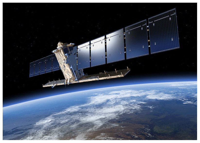
Figure 1Artist's impression of the S-1 satellite; © ESA.
GPS is the only POD observation technique available for Sentinel-1. Assessment of the absolute orbit accuracy is, therefore, difficult. Radar measurements have already successfully been applied for orbit validation of TerraSAR-X and TanDEM-X (Hackel et al., 2018). Schmidt et al. (2018) indirectly validated the Sentinel-1 NTC orbits with radar measurements but did not reach the level of accuracy necessary for absolute orbit validation. The validation of the orbit accuracy can, therefore, only be done by orbit overlap analysis and by comparison to other orbits generated from different institutions. The Copernicus POD Quality Working Group (QWG) is part of the CPOD Service. The member institutions of the QWG deliver independent orbit solutions for all Sentinel satellites using different software packages and different reduced-dynamic orbit determination (Wu et al., 1991) approaches. These alternative orbit solutions are compared in four-month batches to the operational CPOD solutions. The comparisons are published in the Regular Service Review (RSR) reports (https://sentinel.esa.int/web/sentinel/missions/sentinel-1/ground-segment/pod/documentation, last access: 16 March 2020). Based on these RSR comparisons and following detailed investigations (Peter et al., 2017) an erroneous information in the Sentinel-1 satellite geometry could be identified. The Up-component of the GPS antenna phase center offset (PCO) w.r.t. the antenna reference point (ARP) has, therefore, been corrected by 29 mm. The consistency between the CPOD and POD QWG orbit solutions could significantly be improved although systematic differences were still present in particular during the eclipse period from May to August.
S-1A and S-1B satellites are identical in construction. Therefore, estimated orbit parameters allow to indirectly validate the orbit solutions by comparing the estimated parameters such as solar radiation pressure (SRP) coefficient or empirical cycle-per-revolution (CPR) parameters with each other. They are expected not to be exactly the same but they should have the same magnitude.
If the same orbit and observation models are applied for precise orbit determination of the two satellites different results for the estimated orbit parameters might be caused by erroneous satellite geometry, namely center-of-mass (COM) coordinates, GPS ARP coordinates or GPS antenna PCO + PCVs (phase center variations). Antenna offset estimation is a common method to sort out inconsistencies between satellite geometry, observation and orbit models. Luthcke et al. (2003) and Haines et al. (2004) for instance did an offset estimation for Jason-1 by estimating the GPS antenna PCO together with the phase center variations (PCV). Radial orbit accuracy and post-fit observation residuals could significantly be improved. Peter et al. (2017) discussed the interdependency of PCO and PCVs in detail for S-1A. They claimed the necessity of having PCVs available, which do not induce offsets, in particular for satellite missions where such auxiliary data is provided to users with different software packages and different reduced-dynamic or even kinematic orbit determination strategies.
In the study presented here antenna offset estimation means the estimation of the vector from COM of the satellite to the ARP, in most cases the physical mounting point of the GPS antenna. Although a potential error cannot be assigned either to the COM or the ARP or PCO/PCV, the antenna PCO and PCVs are handled separately and are not included into this term in this case.
A main topic of this research is the sensitivity of such antenna offset estimations to orbit and observation modelling for the special case of the Sentinel-1 mission. The two satellites A and B are flying in the same sun-synchronous dawn-dusk orbit (inclination 98.18∘, altitude 693 km) but 180∘ apart. This orbit implies a sun angle over the orbital plane between 58 and 87∘ with an eclipse period of less than 100 d between May and August (see Fig. 2).
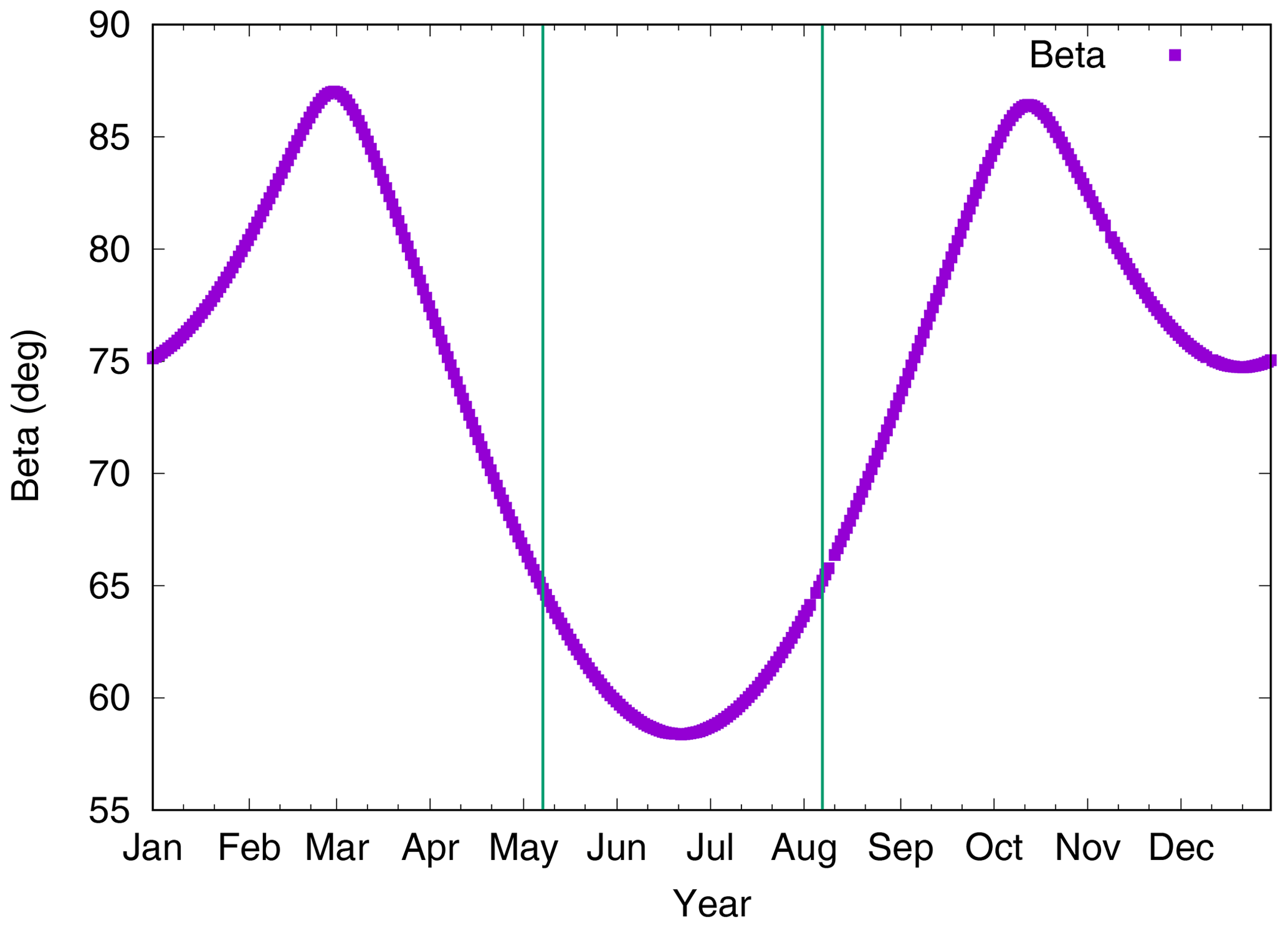
Figure 2Sun angle above the orbital plane (β), eclipse period between lines in the middle of the year.
The solar panels are fixed to an angle of 30∘ with respect to the satellite's z-axis (perpendicular to the SAR antenna face direction and positive in direction of radiation) in the satellite-fixed reference frame (SRF). The xSRF-axis approximately points into the flight direction and the ySRF-direction is the anti-sun direction. In nominal attitude mode (for details see Peter et al., 2017; Fiedler et al., 2005; Miranda, 2005) the satellite bus is tilted approximately by 30∘ with respect to the nadir direction as it is implied in Fig. 1. The GPS antennas are also tilted w.r.t. the satellite bus (Peter et al., 2017) to have the antenna boresight close to zenith direction all the time. The non-gravitational force modelling is done based on a satellite macromodel (box-wing model). The satellite and orbit design implies a strong correlation between SRP modelling and the cross-track component of the orbit. This fact impacts the selection of the orbit parameter setup and also plays an important role when analysing sensitivity of the S-1 antenna offset estimation to orbit and observation modelling.
Considering the complex shape of the Sentinel-1 satellites, the mission and orbit design, the dependency of the offset estimates on the complexity of the satellite macromodel and different orbit parametrizations is analysed. Sophisticated satellite models based on ray tracing considering shadowing effects and multiple reflections proved to be beneficial to satellite macromodels (Haines et al., 2004; Zelensky et al., 2010) for the non-gravitational force modelling. Such a sophisticated Sentinel-1 satellite model has been developed by University College London (UCL, Li et al., 2018), but it is not publicly available and has not yet been validated in S1 POD. Therefore, self-shadowing effects are tried to be considered in the present study by simple assumptions depending on the sun incident angle on the individual satellite surfaces. The satellite macromodel is updated accordingly.
In addition, the improvement in observation modelling, namely the application of single-receiver ambiguity resolution for the Sentinel satellites (Montenbruck et al., 2018a), is also taken into consideration for the analysis presented here. Single-receiver ambiguity resolution has already successfully been applied for other LEO (Low Earth Orbiting) satellites such as GRACE, Jason-1, and Jason-2 (Laurichesse et al., 2009; Bertiger et al., 2010). Montenbruck et al. (2018a) nicely showed the impact of integer ambiguity resolution on the cross-track component of the orbit due to the geometric stiffness given by the fixed ambiguities. The integer ambiguity resolution could be applied for the Copernicus Sentinel-1, -2, and -3 satellites only recently, when the ground segment processing was upgraded to properly resolve half-cycle biases in the carrier phase observations from raw correlator data of the RUAG GPS receivers (Zangerl et al., 2014). This was shown for the first time for Swarm also being equipped with the RUAG GPS receiver (Allende-Alba and Montenbruck, 2016). Full-cycle ambiguities can, fortunately, be generated in a post-processing on ground and ambiguity resolution results were already presented for Swarm in a baseline (Allende-Alba et al., 2017) and in single-receiver processing (Montenbruck et al., 2018b). Results for Sentinel-3A were presented in Montenbruck et al. (2018a).
The sensitivity analysis of the S-1 antenna offset estimation is composed as follows. Section 2 shows the differences in the orbit determination results of the two S-1 satellites. Section 3 describes the different orbit and observation models used, in particular a detailed description of the macromodel update including assumptions on the self-shadowing. The results of the different antenna offset estimations based on the different orbit and observation models are summarised and analysed in Sect. 4. The article is closed with conclusions in Sect. 5.
Part of motivation for this study is that the estimated orbit parameters (e.g., SRP coefficient and empirical CPR parameters) of the two Sentinel-1 satellites show different magnitudes and or systematic signatures, which cannot be explained by other means than different antenna offset vectors of the GPS antennas. The satellites are identical in construction, but of course there are differences in the satellite mass due to the different age of the satellites. The satellite masses change over time, which is documented in the corresponding mass history files available from S-1 FOS (Flight Operations Segment). For instance the satellite masses have been 2145.057 and 2153.622 kg on 11 June 2018 for S-1A and S-1B, respectively. The differences of about 8.5 kg is not very large compared to the absolute mass of the satellites. The satellite mass is used in the non-gravitational force models as scaling factor to model the resulting acceleration. Therefore, the mass is already properly incorporated in the modelling and the SRP coefficient and atmospheric drag scaling factor should not show large differences due to this. Significant differences are, however, present in the center of mass (COM) coordinates of the two satellites. Table 1 lists the corresponding COM coordinates in SRF as of 11 June 2018 in the middle rows. The initial location of the COM is not directly measured but computed based on the location and masses of all spacecraft components. The COM position does also change during mission time, but the changes are very small (about 1 mm yr−1) and restricted to the z-component. Since the launch of the satellites the z-component of the COM of S-1A changed by 8 mm and that of S-1B by 3 mm (status: 8 January 2020). The larger change for S-1A is due to more fuel consumption during the longer lifetime of the satellite and due to the large number of manoeuvres in the first months of the mission to correct the injection error (Martín Serrano et al., 2015; Vasconcelos et al., 2015). The changes of the COM coordinates are also documented in the aforementioned mass history files of the satellites. Table 1 also lists the ARP coordinates of the main and the redundant GPS antennas in the top rows. The values are identical for both S-1 satellites. The redundant antenna is added for completeness but it is not used in the following analysis due to lack of data. The different COM coordinates of the two satellites lead to different antenna offsets (vectors from the COM to the GPS ARPs) for the two satellites (see bottom rows of Table 1, for the main GPS antennas only).
Table 1GPS ARP coordinates for main and redundant antennas (top); COM coordinates (middle) and vectors from COM to the main GPS ARPs (bottom) for the two satellites as of 11 June 2018; all values are given in SRF.
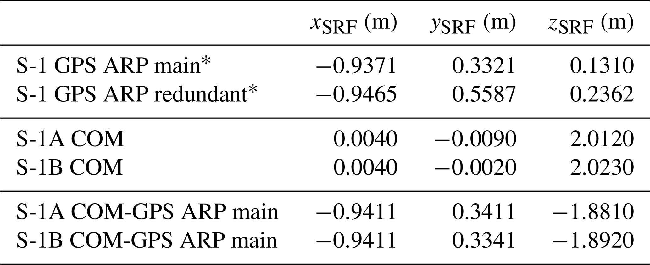
* Note that the GPS ARP coordinates are different to the values documented in Peter et al. (2017). In the meantime an error in the documentation has been detected. Due to operational constraints S-1 operational CPOD orbits are still generated based on the wrong values from Peter et al. (2017); status: 8 January 2020.
Table 2Summary of models and parameters employed for the Sentinel-1 orbit determination.
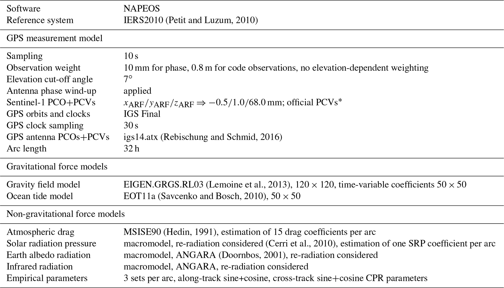
* https://sentinel.esa.int/web/sentinel/technical-guides/sentinel-1-sar/pod/satellite-parameters (last access: 16 March 2020) ⇒ ANTEX file.
Table 2 lists the observation model, orbit model and the parameters used for S-1 orbit determination in this section, basically the settings of the operational S-1 NTC orbit determination at the CPOD Service. Different settings used for the analyses in Sect. 4 are explicitly stated in Table 3. The S-1 macromodel is described in detail in Sect. 3.1.

The estimated orbit parameters from S-1A and S-1B are analysed based on orbit determination results from one year of data (2018). At first, Fig. 3 shows the estimated SRP coefficient. The estimates are different for the two spacecraft and also show seasonal variations. Mean values are 0.94±0.04 and 1.03±0.06 for S-1A and S-1B, respectively. During the eclipse period in the middle of the year (see Fig. 2) the estimated SRP coefficients are closest, but outside the eclipse period the values differ up to 10 % from each other.
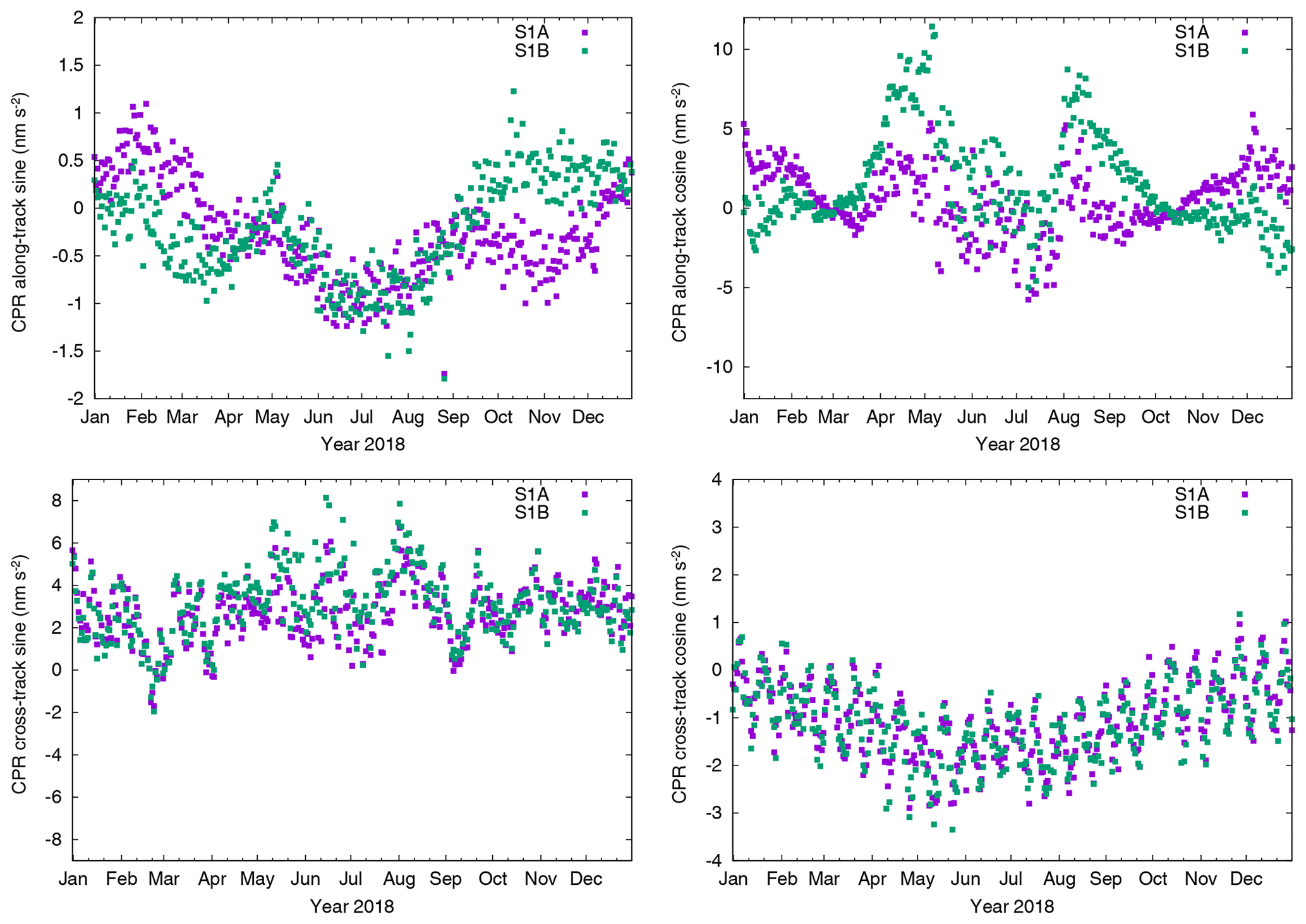
Figure 4 shows the two (sine and cosine) elements of the empirical along-track and cross-track CPR parameters, respectively. Three CPR parameter sets are estimated per orbital arc and the three values of each element are very similar. For simplicity only the elements of the second CPR parameter are shown. It has to be noted that the scale is centered to zero in all four panels but different for the four parameters. The cosine cross-track parameters (bottom right) are very similar for both satellites. They do not exhibit large differences. The sine cross-track parameters (bottom left) are similar outside the eclipse period but during eclipse the values differ by up to 2 nm s−2. The along-track parameters (top row) show differences in both elements, especially outside the eclipse period. The differences grow up to 5 nm s−2 on some days for the cosine along-track element (top right).
To check if the differences in the estimated orbit parameters are due to different antenna offset vectors, the estimation of the y- and z-component of the antenna offset vector has been performed for both satellites. The x-component cannot be estimated for Sentinel-1, because this direction is fully correlated with the along-track component of the state vector. A reliable estimation of the antenna offsets in a reduced-dynamic orbit determination can only be guaranteed when the underlying gravitational and non-gravitational force models are sufficiently good. The radial orbit component is defined by the dynamical models. Any mismodelling does, therefore, directly impact the levelling in radial direction. The cross-track orbit component is also defined by the dynamical models. In the case of Sentinel-1 in the sun-synchronous dawn-dusk orbit this is especially the SRP modelling. That means that the satellite macromodel used for the non-gravitational force models is of high importance for a reliable estimation of the cross-track orbit component. Mismodelled forces should not deteriorate or even falsify the estimates. In the case of Sentinel-1 self-shadowing plays an important role due to the specific shape and orientation of the satellite and should be taken into account for accurate SRP modelling. The impact of using different macromodels with and without taking self-shadowing into account is, therefore, studied for the antenna offset estimation. In addition, the single-receiver ambiguity resolution has been considered in the GPS observation modelling. The improvement, which mainly impacts the cross-track orbit component due to the geometric stiffness given by the fixed carrier-phase ambiguities (Montenbruck et al., 2018a), is studied as well for the antenna offset estimation.
The processing of the data used for this study is based on the model and parameter settings given in Table 2. The settings of the solutions used for the antenna offset estimation are only partly different and the differences to the settings in Table 2 are mentioned in Table 3 (right column).

Common for all solutions is that no PCVs are used, because it shall be avoided to introduce any possible implicit offsets from the PCVs (see Peter et al., 2017). The y- and z-component of the antenna offsets are estimated in all solutions and the corresponding a priori values are the differences between the main GPS ARP and COM coordinates (see bottom rows of Table 1). It is also common to all solutions that CNES-CLS (Loyer et al., 2012) Final orbit and clock products are used for the processing instead of the IGS Final orbit and clock products. Single-receiver ambiguity-fixing is done for solutions A–F based on the available widelane satellite biases from CNES-CLS together with corresponding GPS satellite clocks having included the narrowlane phase biases (Laurichesse et al., 2009). Solution C is considered as standard solution, because it uses the macromodel described in Table 4 and reasonable parameter settings for the antenna offset estimation. To show the impact of the carrier-phase ambiguity-fixing on the offset estimation a corresponding ambiguity-float solution is also computed (solution CFL). The entire year 2018 is processed for both satellites generating several solutions listed in Table 3. Solutions D and E are added to show the impact of obviously insufficient models on the antenna offset estimations.
Table 4Sentinel-1 macromodel, instantaneous re-radiation (Cerri et al., 2010) used for all panels except solar array front and back.
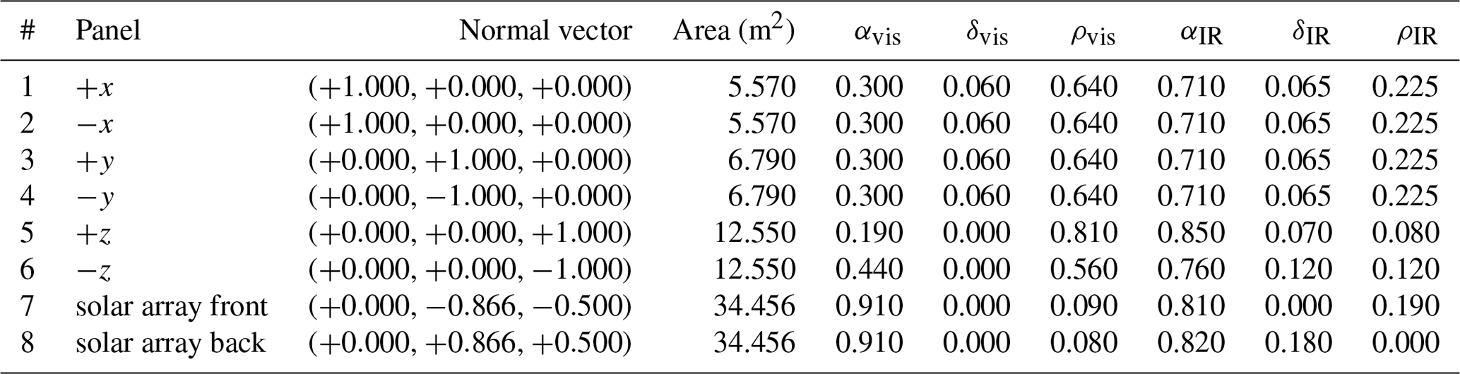
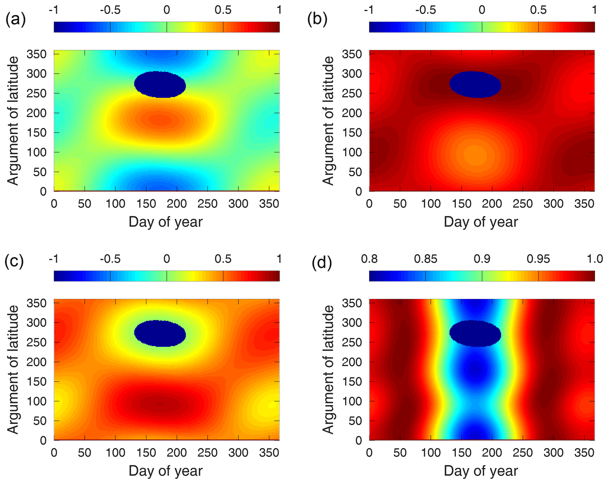
Figure 5cos (θ) values for each day of a year (x-axis) depending on the argument of latitude (y-axis); (a) −x, (b) : −y, (c) −z, (d) solar array.
3.1 Sentinel-1 macro-model
Modelling of accelerations due to atmospheric drag, SRP and ERP is done based on a macromodel of the Sentinel-1 satellite. The macromodel consists of eight planes. The surface area and normal vector in SRF of each panel are given along with the visual (vis) and infrared (IR) optical properties in Table 4. The macromodel is compiled based on information available to the Copernicus POD Service (https://sentinel.esa.int/web/sentinel/missions/sentinel-1/ground-segment/pod/documentation, last access: 16 March 2020), Sentinel-1 properties for GPS POD. Some assumptions are taken, e.g., the ratio of MLI (multi-layer isolation) and radiator surfaces on the satellite bus. The spacecraft bus and the SAR antenna are described by the first six panels in -directions. The last two panels are the sum of the front and back of the two solar panels, respectively. In the case of Sentinel-1 the solar panels are not continuously rotating to have the optimum angle towards the sun. The solar panels are fixed at a 30∘ angle with respect to the z-axis of the SRF during nominal operations (Peter et al., 2017). The S-1 macromodel is based on length, width, and height measures of the satellite bus, the SAR antenna and the solar panels. No sticking out instruments like star cameras, GPS or telemetry antennas are considered for the model. The uncertainty level of the macromodel areas is at about 5 %. Solution D uses an older S-1 macromodel, which considered smaller areas for the ±y-surfaces and the solar arrays, see Table 3. Although present in the documentation the thickness of the SAR antenna (0.2 m thick on a length of 12.3 m, more than a third of the entire y surface) was overlooked for the ±y-surfaces as well as the triangle mountings of the solar arrays (about 10 % of the solar array area). The old macromodel did only take the reduced areas into account.
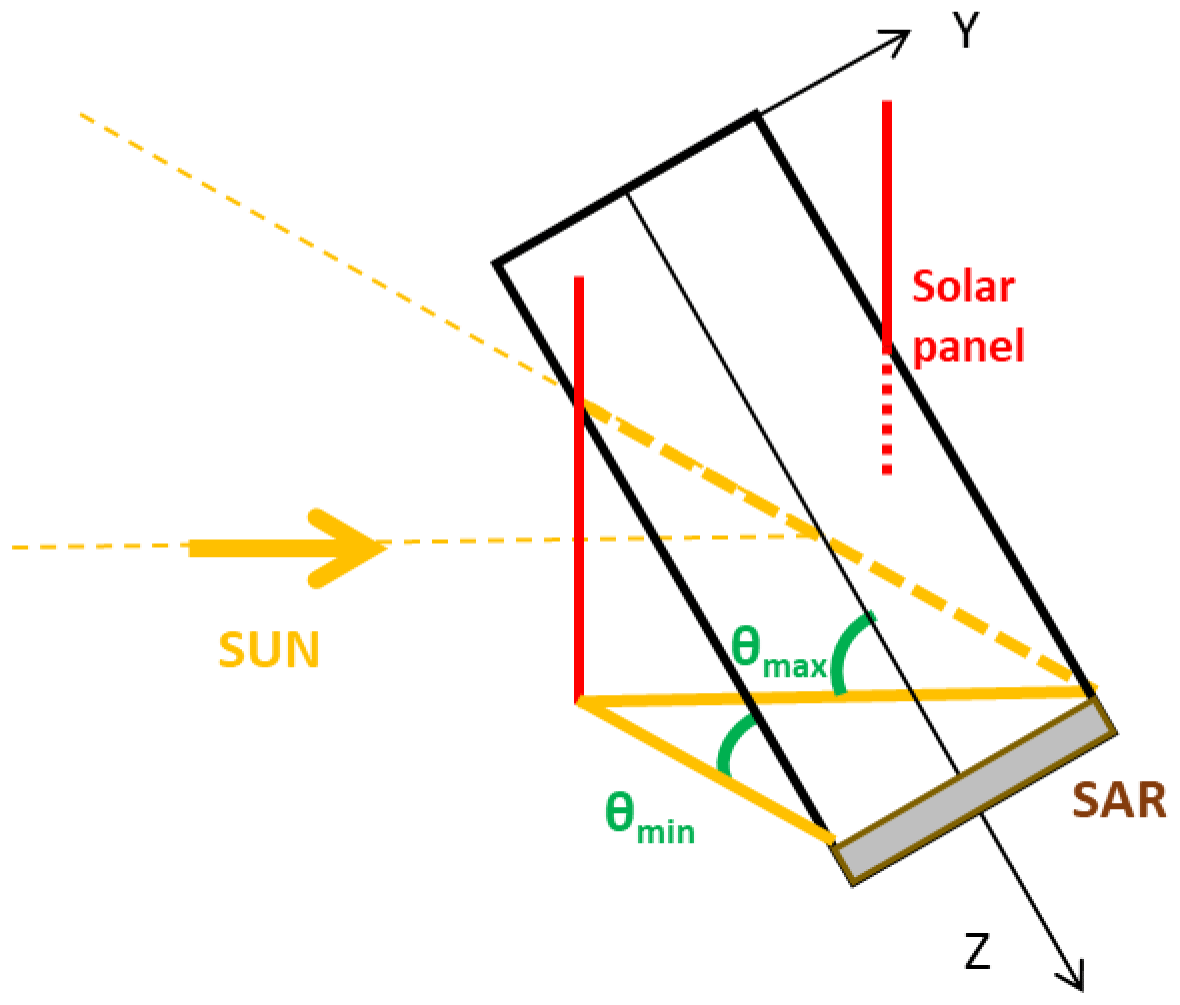
Figure 6Schematic drawing of shadowing assumptions of solar array on backside of SAR antenna (−z surface).
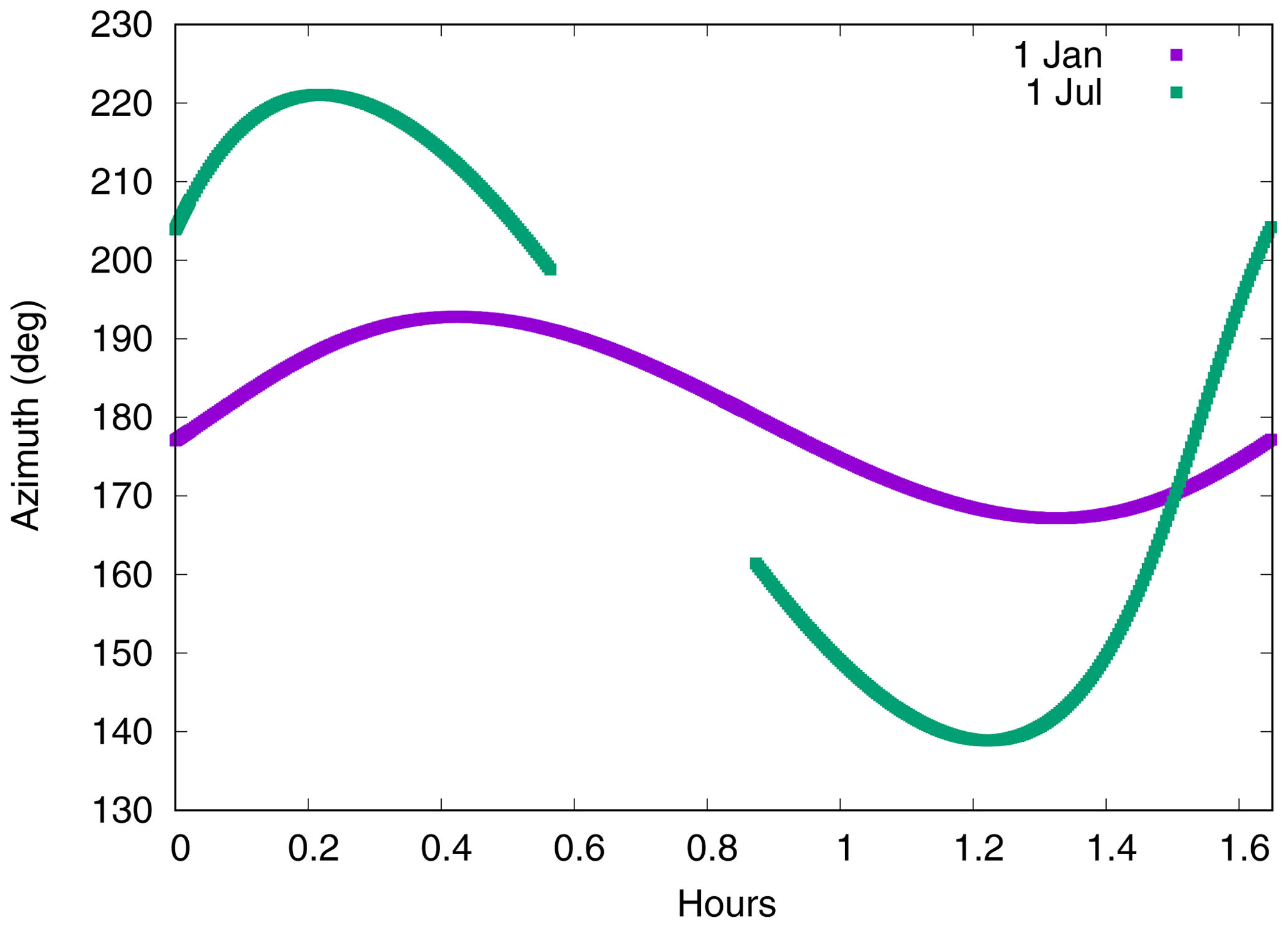
Figure 7Azimuth angle of the sun in SRF (+ySRF corresponds to 0∘) for approximately one orbital revolution on two example days, 1 January and 1 July.

3.2 Self-shadowing updates for Sentinel-1 macromodel
A simple box(-wing) model cannot give full consideration to the complex shape of Sentinel-1, in particular not to shadowing effects, e.g., by one of the solar arrays to the backside of the SAR antenna. Therefore, an update of the macromodel is developed to consider part of the shadowing effects. The simple shadowing assumptions have proven to be beneficial for the SRP modelling especially during the eclipse period of the Sentinel-1 satellite (Peter et al., 2018). The first step to develop the box-wing model updates is to analyse the sun incident angles on the individual satellite surfaces. The angle θ is the angle between the normal vector of a surface and the direction of the sun. The values of cos (θ) are analysed, because these values are used as scaling factors for computing the acceleration due to SRP (and other non-gravitational forces) on the individual surfaces. If cos (θ)=1 the sun is perpendicular to the surface meaning the maximum solar radiation is effective on this particular surface. If the values are negative, the sun is not shining on the surface.
Figure 5 shows the values for cos (θ) for the −x (panel a), −y (panel b), −z (panel c), and for the solar array (panel d) for each day of the year (x-axis) and depending on the argument of latitude of the satellite (y-axis). Except for the solar array (0.8…1.0) the values range from . The values for the corresponding surfaces in the -directions and the back of the solar array are just the same but with opposite sign. That means that the +y and +z-surfaces and the solar array back are never in sunlight. The part of the orbit, which is in eclipse in the middle of the year can be noticed as dark blue ellipse in each plot at argument of latitude between 250 and 300∘. No surface is in sunlight during the eclipse transitions of course. The values for the solar array (bottom right) indicate that the sun is always close to perpendicular to the solar cells. During eclipse period the values are smallest. Similar to the solar array, the −y-surface (top right) is also always illuminated by the sun. The −x-surface (top left) shows the largest variations also during one orbital revolution. Both x-surfaces do, therefore, change from sun to shadow during all orbital revolutions. The −z-surface is partly the backside of the SAR antenna and this surface is also always in sunshine. Based on the analysis of cos (θ) the geometry of the Sentinel-1 spacecraft is studied in more detail for shadowing effects.
Figure 6 shows a schematic view of the spacecraft. The xSRF-axis is pointing into the paper. The spacecraft is tilted by 30∘, which corresponds to the nominal attitude configuration. The sun is always coming from the “left” in this case. Due to the asymmetric mounting of the solar panels on the satellite body only one of the panels can shadow the backside of the SAR antenna. This shadowing is explained based on the drawing in Fig. 6. The angles θmin and θmax indicate the sun incident angles on the −z-surface, which are the limits for the shadowing of the solar panel on the backside of the SAR antenna. When the sun is between these two θ angles the SAR antenna is gradually shaded. The shadowing starts with ∘ and is at a maximum with ∘. Based on Fig. 5 it is known that θ=60∘ is also the maximum possible angle for the −z-surface. It is assumed that the shadowing grows with a linear gradient of cos (θ). At maximum the entire backside of the SAR antenna is shaded on this side of the satellite (42.86 % of the −z-area). It is clear that the real shadowing function is more complicated and not only dependent on θ. The azimuth of the sun incident angle does also have an impact. Figure 7 shows the azimuth of the sun incident angle in SRF on two example days, 1 January and 1 July, for approximately one orbital revolution. The amplitudes are ±10∘ on 1 January and ±40∘ on 1 July with respect to an azimuth of 180∘, which corresponds to the −y-direction. The gap in the data of 1 July is due to the eclipse. In the case of the −z-surface an azimuth variation of 40∘ accounts to about 3.5 % of the −z-area. This is less than 10 % of the maximum shaded area of the −z-surface. For the sake of simplicity the azimuth of the sun incident angle is neglected for this study.
Table 5 lists the shadowing conditions applied for Sentinel-1. In addition to the largest shadowing of the solar array on the −z-surface, the shadowing of the −x-surface by the solar array and of the other solar array by the satellite body is considered as well. The angles and maximal shadowed areas for these additional shadowings are derived from corresponding considerations as shown in Fig. 6. The condition to consider the shadowing of the solar panel by the satellite body is the same as for the shadowing of the −x-surface.
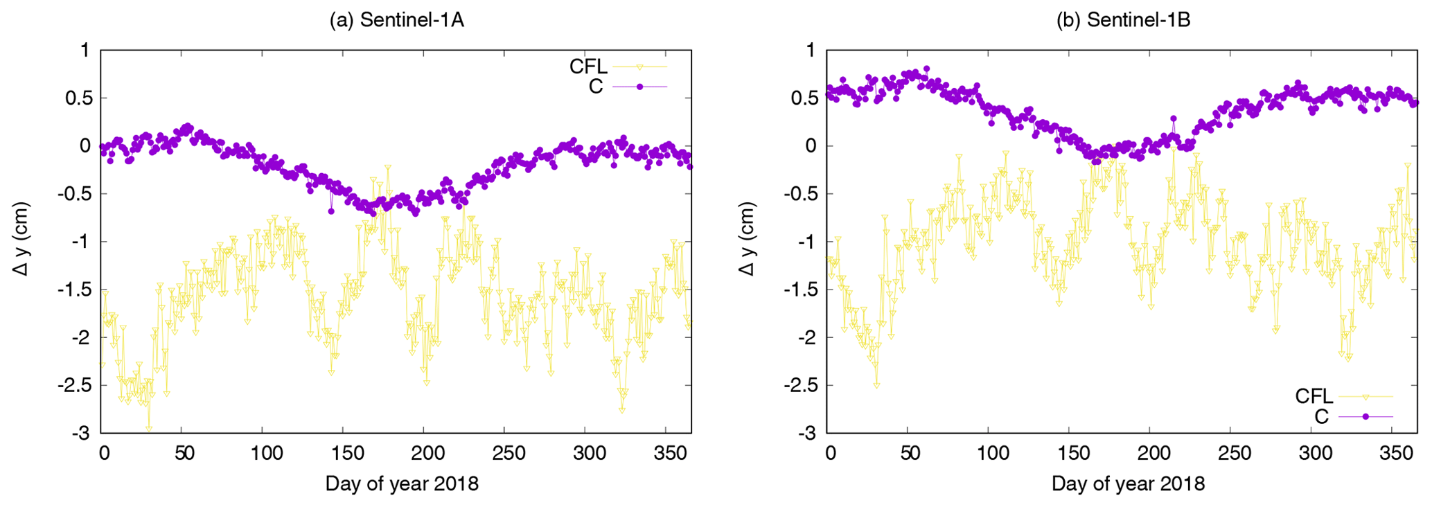
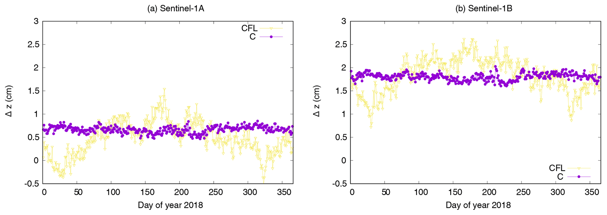
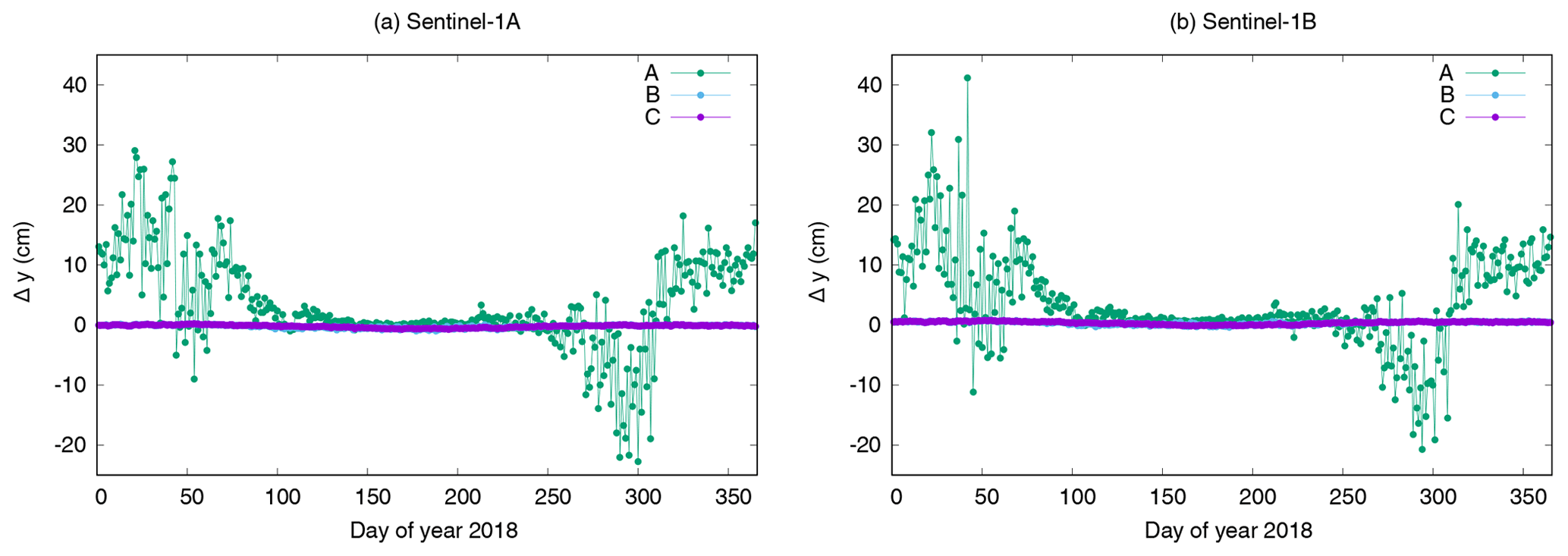
The results of the antenna offset estimations from the different solution types listed in Table 3 are presented in this section. The estimates of the y- and z-component of the antenna offsets (delta to the a priori values from Table 1) are displayed in Figs. 8–13 for both Sentinel-1 satellites for the year 2018. The estimates for S-1A are always visible in panels (a) and those for S-1B always in panels (b). Table 6 lists the corresponding mean values and standard deviations for all solutions and all estimates.

At first, the impact of the carrier-phase ambiguity-fixing on the offset estimation is shown based on the comparison of the offset estimates of solutions CFL and C (Figs. 8 and 9). The advantage of the ambiguity-fixing becomes clearly visible in the results. The offset estimates for the C solution are less noisy than those for the CFL solution. The standard deviations of the estimates range between 0.7 and 2.4 mm for the C solution compared to a range between 3.7 and 4.9 mm for the CFL solution. In particular the Δy estimates are significantly different for the two solutions, 1.77 cm for S-1A and 1.37 cm for S-1B. The cross-track orbit direction benefits most due to the tight constrain given by the fixed ambiguities (Montenbruck et al., 2018a). In the case of S-1 the cross-track orbit direction is highly correlated to the modelling of the SRP due to the sun-synchronous dawn-dusk orbit. The SRP modelling is fixed by the S1 macromodel and the corresponding fixed radiation pressure coefficient for solutions C and CFL. With float ambiguities (CFL) any cross-track shift due to mismodelled SRP or wrong antenna offsets goes either into the float ambiguities or into the offset estimates (mainly into the y-offset due to the 30∘ tilted satellite bus). With fixed ambiguities (C) any cross-track shift is mapped to the offset estimates. The z-offset is also partly affected by this due to the tilted satellite bus. Any shift in radial direction affects both offset estimates, but mainly the z-component. In contrary to the cross-track direction the radial orbit component is fully determined by the dynamical model. Whether carrier-phase ambiguities are estimated as float values or fixed to their integer values does not significantly impact the mean radial orbit component. This can be noticed when comparing the estimated z-offsets. The difference between solution C and CFL is 1.8 and 0.3 mm in Δz for S-1A and S-1B, respectively. The standard deviations of the z-offset estimates do, however, benefit significantly from the ambiguity-fixing (3.7 mm vs. 0.7 mm for S-1A and 3.8 mm vs. 0.8 mm for S-1B). Solution C is displayed in all following plots as well, because it is considered as standard solution. Thus the differences to this solution can always directly be seen.
Figures 10 and 11 show the estimates for solutions A, B, and C. It is obvious that the estimation of the antenna offsets together with estimating the SRP coefficient (solution A) shows very large deviations in the estimates during the non-eclipse period of the satellites. The correlation between the SRP coefficient and in particular the y-component of the antenna offset causes these large deviations and it is not recommended at all to do a common estimation of these coefficients. The results of solution A also reveal the special case of Sentinel-1. Except during the eclipse period from beginning of May until beginning of August, the satellites are in full sun for the entire orbital revolution. The decorrelation of the SRP coefficient and constant empirical orbit parameters acting in cross-track direction is, therefore, very difficult. Thus the SRP coefficient may also absorb other modelling deficiencies than intended for.
The SRP coefficient is, therefore, fixed to 1.0 for all other solutions. The antenna offset estimates for solutions B and C are very similar for the individual satellites. The estimates differ in the sub-mm range. The standard deviations of the y-offset estimates from solution B are insignificantly larger than those of solution C, but for the z-component the estimates for solution C are much more precise than for solution B. This means that the additional estimation of sine and cosine CPR parameters does not harm the solution. It gives less noisy estimates and thus for the following solutions the estimation of the sine and cosine CPR parameters is kept. The results from solutions B and C already show that the offset estimates are different between S-1A and S-1B. The difference between S-1A and S-1B in Δy is 0.55 cm whereas the difference in Δz is 1.34 cm.
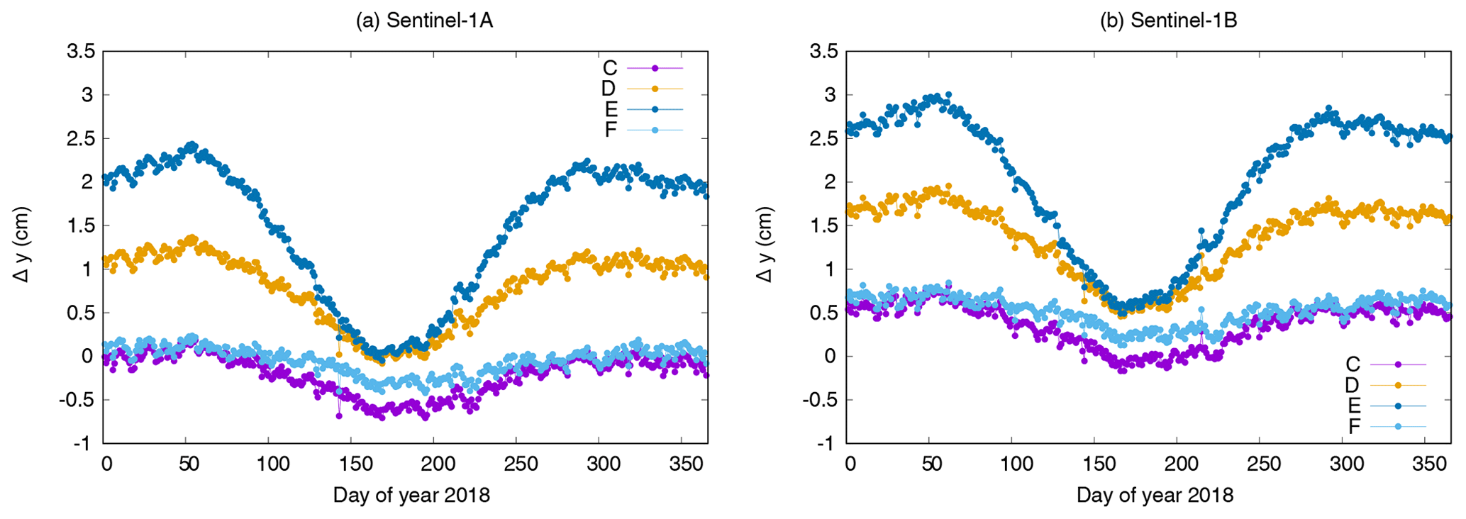
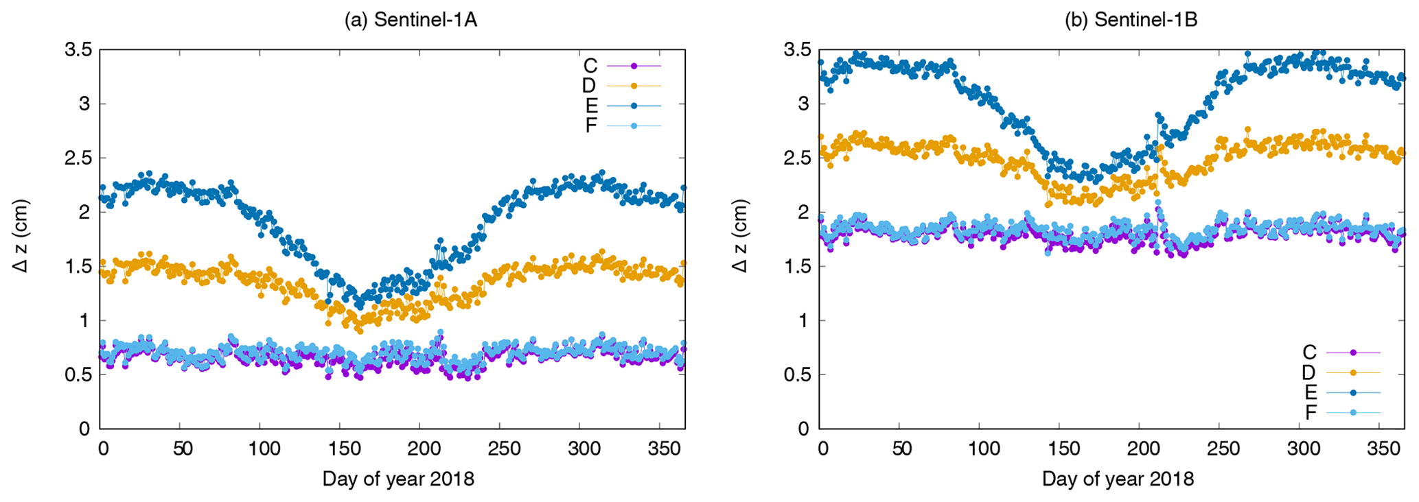
The antenna offset estimates of solutions C–F are shown in Figs. 12 and 13. The values are closest for all solutions during eclipse period but for the rest of the year the differences grow up to 1.5 cm. Solution E using the constant area for the SRP modelling differs most from Solution C. The impact of the insufficient modelling is obvious. The older macromodel used for Solution D also leads to differences up to 1 cm in the mean value (Δy S-1B).
Table 6Mean and standard deviation (cm) of Δy and Δz antenna offset estimates.

Table 7Corrected displacement vectors between main GPS ARP and COM for S-1A and S-1B (based on solution F).
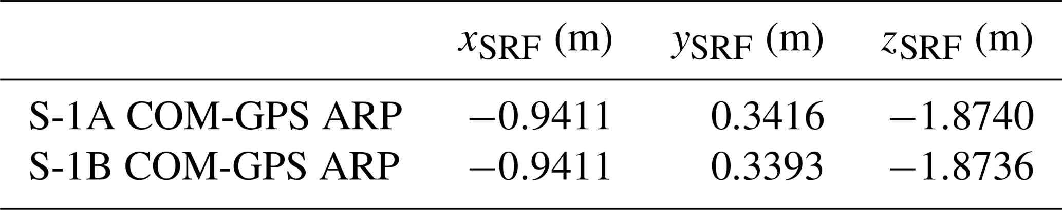
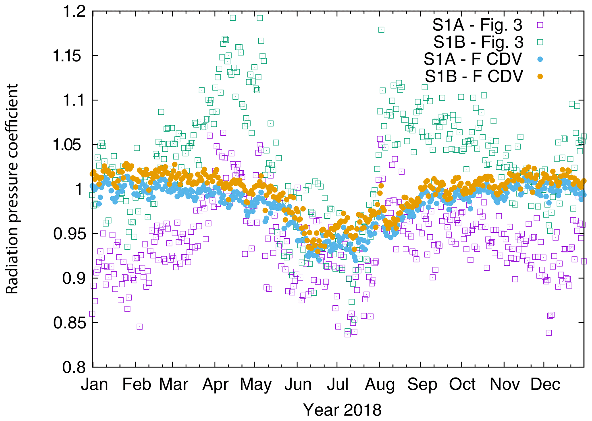
Figure 14Estimated SRP coefficient for both Sentinel-1 satellites, original and F CDV solution.
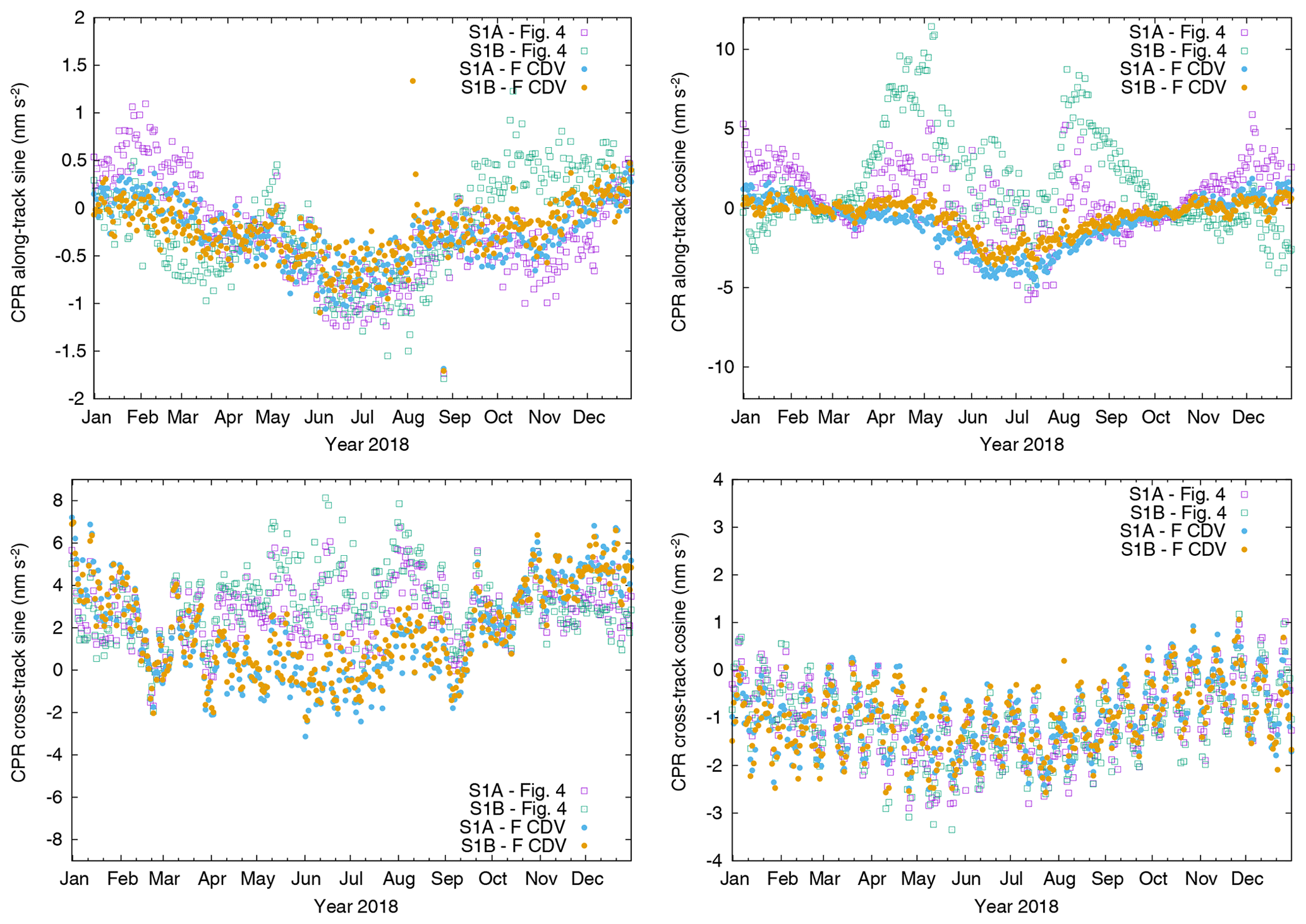
Figure 15Estimated CPR parameters for both Sentinel-1 satellites, original and F CDV solution.
Solution F shows equivalent results as solution C for the z-component, only sub-mm differences in the estimates are present. The differences in the y-component are larger with 0.26 cm for S-1A and 0.15 cm for S-1B. Additionally, the standard deviations get slightly smaller from 0.23 to 0.15 cm for S-1A and from 0.24 to 0.17 cm for S-1B. The inclusion of simplified shadowing effects has a small impact but the lower standard deviations of the y-offset estimates confirm a better consistency of the updated macromodel with the fixed SRP coefficient (1.0) and the real conditions.
When applying the estimates of solution F to the a priori antenna offset values from Table 1 the displacement vectors between GPS ARP and COM of the individual satellites become very similar within 1–2 mm (Table 7). It cannot be assessed if the corrections to the displacement vector are caused by wrong COM coordinates or wrong ARPs.
To conclude the analysis the orbit determination (as shown in Sect. 2) has been repeated with the corrected displacement vectors between main GPS ARP and COM for both satellites, respectively, and with the modelling of solution F. In accordance with the original orbit determination settings the SRP coefficient is estimated and the antenna offset estimation is not done (solution ID: F CDV). Figure 14 shows the estimated SRP coefficient of this solution together with the SRP coefficient estimates from the original solution (Fig. 3). The estimates are now closer to each other for the two satellites. The SRP coefficients of the ambiguity-fixed solutions (light blue and orange) are very similar for both satellites and close to 1.0, which is in line with the SRP coefficient fixed to 1.0 for the antenna offset estimation. Only during eclipse period, the estimates gradually drop to values around 0.95. This might hint to still remaining satellite model deficiencies for the SRP modelling during eclipse. Figure 15 shows the four time series of the different CPR parameters for the final ambiguity-fixed orbit solutions using the corrected displacement vectors and for the original solution (Fig. 4). Except for the cross-track cosine parameter (bottom right) all other parameters show significant differences to the original solution. The estimated parameters are also closer to each other for the two satellites. In particular the two along-track parameters (top row) have a lower dispersion than the values for the original solution.
The corrected displacement vectors between COM and GPS ARP lead to consistent estimated orbit parameters of S-1A and S-1B, which is expected for the two identically constructed satellites.
The Copernicus Sentinel-1 mission consists of two identically constructed satellites. Nevertheless, different orbit parameter estimates are present in the precise orbit determination results making an antenna offset estimation necessary. Due to the sun-synchronous orbit and the complex satellite design, the large solar arrays mounted on the two sides of the satellite bus and the long SAR antenna partly shaded by one of the solar panels, the sensitivity of the antenna offset estimation to orbit modelling has been studied. Several solutions with different macromodels for the satellite are performed. Additionally, the observation modelling was updated by applying single-receiver ambiguity resolution.
All the different solutions for antenna offset estimation show the sensitivity of the estimates on the orbit modelling and on the observation modelling. Introducing carrier phase ambiguity fixing significantly improves the antenna offset estimates due to the stiffer solution resulting in less noisy estimates. In particular the y-component mainly representing the cross-track orbit direction benefits most. Highly insufficient satellite macromodels (solutions D and E) have significant negative impact on the antenna offset estimates.
The first main conclusion of this study is the necessity of performing carrier phase ambiguity resolution to stabilise in particular the cross-track orbit component. The second main conclusion is that the orbit modelling, for Sentinel-1 in particular the SRP modelling, is of utmost importance to get reliable antenna offset estimates. Finally, resulting antenna offset estimates for S-1A and S-1B lead to consistent displacement vectors from COM to the main GPS ARP of the individual satellites and to consistent estimated orbit parameters in the orbit determination results.
The Sentinel-1 GNSS data are available on the Copernicus Open Access Hub (https://scihub.copernicus.eu ⇒ POD Hub, ESA, 2020a). Support information for the processing is available on https://sentinel.esa.int/web/sentinel/missions/sentinel-1/ground-segment/pod/documentation (ESA, 2020b).
HP designed the study, carried out the data processing, interpreted the results and wrote the manuscript. JF contributed to discussions and to the final manuscript. PF contributed to the final manuscript.
The authors declare that they have no conflict of interest.
This article is part of the special issue “European Geosciences Union General Assembly 2019, EGU Geodesy Division Sessions G1.1, G2.4, G2.6, G3.1, G4.4, and G5.2”. It is a result of the EGU General Assembly 2019, Vienna, Austria, 7–12 April 2019.
The Copernicus POD Service is financed under ESA contract no. 4000108273/13/1-NB, which is gratefully acknowledged. The work performed in the frame of this contract is carried out with funding by the European Union. The views expressed herein can in no way be taken to reflect the official opinion of either the European Union or the European Space Agency. The authors also acknowledge the work done by the joint CNES/CLS analysis center of the IGS, which provides the GPS orbit, clock and bias products used for the ambiguity-fixed Sentinel-1 orbit solutions in this study. The provision of combined GPS orbit and clock products by the IGS is also greatly appreciated.
This paper was edited by Adrian Jaeggi and reviewed by two anonymous referees.
Allende-Alba, G. and Montenbruck, O.: Robust and precise baseline determination of distributed spacecraft in LEO, Adv. Space Res., 57, 46–63, https://doi.org/10.1016/j.asr.2015.09.034, 2016. a
Allende-Alba, G., Montenbruck, O., Jäggi, A., Arnold, D., and Zangerl, F.: Reduced-dynamic and kinematic baseline determination for the Swarm mission, GPS Sol., 21, 1275–1284, https://doi.org/10.1007/s10291-017-0611-z, 2017. a
Aschbacher, J. and Milagro-Pérez, M.: The European Earth monitoring GMES programme: Status and perspectives, Remote Sens. Environ., 120, 3–8, https://doi.org/10.1016/j.rse.2011.08.028, 2012. a
Bertiger, W., Desai, S. D., Haines, B., Harvey, N., Moore, A. W., Owen, S., and Weiss, J. P.: Single receiver phase ambiguity resolution with GPS data, J. Geodesy, 84, 327–337, https://doi.org/10.1007/s00190-010-0371-9, 2010. a
Cerri, L., Berthias, J., Bertiger, W. I., Haines, B. J., Lemoine, F. G., Mercier, F., Ries, J. C., Willis, P., Zelensky, N. P., and Ziebart, M.: Precision orbit determination standards for the Jason series of altimeter missions, Marine Geod., 33, 379–418, https://doi.org/10.1080/01490419.2010.488966, 2010. a, b
Doornbos, E.: Modeling of non-gravitational forces for ERS-2 and ENVISAT, PhD Thesis, Delft University of Technology, Delft, 2001. a
ESA: Sentinel-1 GNSS data, available at: https://scihub.copernicus.eu, last access: 16 March 2020a. a
ESA: Documentation – POD, Sentinel Online, available at: https://sentinel.esa.int/web/sentinel/missions/sentinel-1/ground-segment/pod/documentation, last access: 16 March 2020b. a
Fernández, J., Escobar, D., Águeda, F., and Féménias, P.: Sentinels POD Service Operations, SpaceOps 2014 Conference, SpaceOps 2014 Conference, 5–9 May 2014, Pasadena, CA, https://doi.org/10.2514/6.2014-1929, 2014. a
Fernández, J., Escobar, D., Ayuga, F., Peter, H., and Féménias, P.: Copernicus POD Service Operations, in: Proceedings of the Sentinel-3 for Science Workshop, 2–5 June 2015, Venice, Italy, 2015. a
Fiedler, H., Börner, E., Mittermayer, J., and Krieger, G.: Total Zero Doppler Steering – A New Method for Minimizing the Doppler Centroid, IEEE Geosci. Remote S., 2, 141–145, https://doi.org/10.1109/LGRS.2005.844591, 2005. a
Fletcher, K. (Ed.): Sentinel-1: ESA's Radar Observatory Mission for GMES Operational Services, ESA SP-1322/1, ESA Communications, Noordwijk, the Netherlands, ISBN 978-92-9221-418-0, 2012. a
Flohrer, C., Otten, M., Springer, T., and Dow, J.: Generating precise and homogeneous orbits for Jason-1 and Jason-2, Adv. Space Res., 48, 152–172, https://doi.org/10.1016/j.asr.2011.02.017, 2011. a
GMES Sentinel-1 Team, GMES Sentinel-1 System Requirements Document, ES-RS-ESA-SY-0001, available at: http://emits.sso.esa.int/emits-doc/5111-A-S1-SRD.pdf (last access: 16 March 2020), 2006. a
Hackel, S., Gisinger, Ch., Balss, U., Wermuth, M., and Montenbruck, O.: Long-Term Validation of TerraSAR-X and TanDEM-X Orbit Solutions with Laser and Radar Measurements, Remote Sens., 10, 762, https://doi.org/10.3390/rs10050762, 2018. a
Haines, B., Bar-Sever, Y., Bertiger, A., Desai, S., and Willis, P.: One-Centimeter Orbit Determination for Jason-1: New GPS-Based Strategies, Mar. Geod., 27, 299–314, https://doi.org/10.1080/01490410490465300, 2004. a, b
Hedin, A. E.: Extension of the MSIS thermosphere model into the middle and lower atmosphere, J. Geophys. Res., 96, 1159–1172, https://doi.org/10.1029/90JA02125, 1991. a
Laurichesse, D., Mercier, F., Berthias, J.-P., Broca, P., and Cerri, L.: Integer Ambiguity Resolution on Undifferenced GPS Phase Measurements and Its Application to PPP and Satellite Precise Orbit Determination, Navigation, 56, 135–149, https://doi.org/10.1002/j.2161-4296.2009.tb01750.x, 2009. a, b
Lemoine, J.-M., Bruinsma, S., Gégout, P., Biancale, R., and Bourgogne, S.: Release 3 of the GRACE gravity solutions from CNES/GRGS, Geophys. Res. Abstr., EGU2013-11123, EGU General Assembly 2013, Vienna, Austria, 2013. a
Li, Z., Ziebart, M., Bhattarai, S., Harrison, D., and Grey, S.: Fast solar radiation pressure modelling with ray tracing and multiple reflections, Adv. Space Res., 61, 2352–2365, https://doi.org/10.1016/j.asr.2018.02.019, 2018. a
Loyer, S., Perosanz, F., Mercier, F., Capdeville, H., and Marthy, J.-C.: Zero-difference GPS ambiguity resolution at CNES-CLS IGS analysis center, J. Geodesy, 86, 991, https://doi.org/10.1007/s00190-012-0559-2, 2012. a
Luthcke, S. B., Zelensky, N., Rowlands, D. D., Lemoine, F. G., and Williams, T. A.: The 1-Centimeter Orbit: Jason-1 Precision Orbit Determination Using GPS, SLR, DORIS, and Altimeter Data, Mar. Geod., 26, 399–421, https://doi.org/10.1080/714044529, 2003. a
Martín Serrano, M. A., Catania, M., Sánchez, J., Vasconcelos, A., Kuijper, D., and Marc, X.: Sentinel-1A Flight Dynamics LEOP Operational Experience, Proceedings 25th International Symposium on Space Flight Dynamics – 25th ISSFD, October 2015, Munich, Germany, 2015. a
Miranda, N.: Sentinel-1 Instrument Processing Facility, Technical Note, ESA-EOPG-CSCOP-TN-0004, available at: https://sentinel.esa.int/documents/247904/1653440/Sentinel-1-IPF_EAP_Phase_correction (last access: 16 March 2020), 2005. a
Montenbruck, O., Hackel, S., and Jäggi, A.: Precise orbit determination of the Sentinel-3A altimetry satellite using ambiguzity-fixed GPS carrier phase observations, J. Geodesy, 92, 711–726, https://doi.org/10.1007/s00190-017-1090-2, 2018a. a, b, c, d, e
Montenbruck, O., Hackel, S., van den Ijssel, J., and Arnold, D.: Reduced dynamic and kinematic precise orbit determination for the Swarm mission from 4 years of GPS tracking, GPS Sol., 22, 647, https://doi.org/10.1007/s10291-018-0746-6, 2018b. a
Peter, H., Jäggi, A., Fernández, J., Escobar, D., Ayuga, F., Arnold, D., Wermuth, M., Hackel, S., Otten, M., Simons, W., Visser, P., Hugentobler, U., and Féménias, P.: Sentinel-1A – First precise orbit determination results, Adv, Space Res., 60, 879–882, https://doi.org/10.1016/j.asr.2017.05.034, 2017. a, b, c, d, e, f, g, h
Peter, H., Fernández, J., and Féménias, P.: Improved box-wing modelling for the low Earth orbiting Sentinel satellites, presented in session PSD.1 at 42nd COSPAR Scientific Assembly, 14–22 July 2018, Pasadena, CA, USA, available at: https://www.cospar-assembly.org/abstractcd/COSPAR-18 (last access: 16 March 2020), 2018. a
Petit, G. and Luzum, B.: IERS Conventions (IERS Technical Note 36), Verlag des Bundesamts für Kartographie and Geodäsie, Frankfurt am Main, Germany, 179 pp., Paperback, ISBN 3-89888-9898-6, 2010. a
Rebischung, P. and Schmid, R.: IGS14/igs14.atx: a new framework for the IGS products, AGU Fall meeting, San Francisco, CA, G41A-0998, 2016. a
Savcenko, R. and Bosch, W.: EOT11a – Empirical Ocean Tide Model from Multi-Mission Satellite Altimetry, Deutsches Geodätisches Forschungsinstitut, Munich, Report No. 89, 49 pp., hdl:10013/epic.43894.d001, 2010. a
Schmidt, K., Reimann, J., Tous Ramon, N., and Schwerdt, M.: Geometric Accuracy of Sentinel-1A and 1B Derived from SAR Raw Data with GPS Surveyed Corner Reflector Positions, Remote Sensing, 10, 523, https://doi.org/10.3390/rs10040523, 2018. a
Springer, T., Dilssner, F., and Escobar, D.: NAPEOS: The ESA/ESOC Tool for Space Geodesy, Geophys. Res. Abstr., EGU2011-8287, EGU General Assembly 2011, Vienna, Austria, 2011. a
Torres, R., Snoeij, P., Geudtner, D., Bibby, D., Davidson, M., Attema, E., Potin, P., Rommen, B., Floury, N., Brown, M., Navas Traver, I., Deghaye, P., Duesmann, B., Rosich, B., Miranda, N., Bruno, C., L'Abbate, M., Croci, R., Pietropaolo, A., Huchler, M., and Rostan, F.: GMES Sentinel-1 mission, Remote Sens. Environ., 120, 9–24, https://doi.org/10.1016/j.rse.2011.05.028, 2012. a
Vasconcelos, A., Martín Serrano, M. A., Sánchez, J., Kuijper, D., and Marc, X.: Sentinel-1 Reference Orbit Acquisition Manoeuvre Campaign, Proceedings 25th International Symposium on Space Flight Dynamics – 25th ISSFD, October 2015, Munich, Germany, 2015. a
Wu, S. C., Yunck, T. P., and Thornton, C. L.: Reduced-dynamic technique for precise orbit determination of low Earth satellites, J. Guid. Control. Dynam., 14, 24–30, https://doi.org/10.2514/3.20600, 1991. a
Zangerl, F., Griesauer, F., Sust, M., Montenbruck, O., Buchert, B., and Garcia, A.: SWARM GPS precise orbit determination receiver initial in orbit performance evaluation, in: Proceedings ION GNSS+, Institute of Navigation, 8–12 September 2014, Tampa, Florida, 1459–1468, 2014. a
Zelensky, N. P., Lemoine, F. G., Ziebart, M., Sibthorpe, A., Willis, P., Beckley, B. D., Klosko, S. M., Chinn, D. S., Rowlands, D. D., Luthcke, S. B., Pavlis, D. E., and Luceri, V.: DORIS/SLR POD modeling improvements for Jason-1 and Jason-2, Adv. Space Res., 46, 1541–1558, https://doi.org/10.1016/j.asr.2010.05.008, 2010. a