 | 08 Nov 2019
Reservoir-scale transdimensional fracture network inversion
Márk Somogyvári
Michael Kühn
Sebastian Reich
The Waiwera aquifer hosts a structurally complex geothermal groundwater system, where a localized thermal anomaly feeds the thermal reservoir. The temperature anomaly is formed by the mixing of waters from three different sources: fresh cold groundwater, cold seawater and warm geothermal water. The stratified reservoir rock has been tilted, folded, faulted, and fractured by tectonic movement, providing the pathways for the groundwater. Characterization of such systems is challenging, due to the resulting complex hydraulic and thermal conditions which cannot be represented by a continuous porous matrix.
By using discrete fracture network models (DFNs) the discrete aquifer features can be modelled, and the main geological structures can be identified. A major limitation of this modelling approach is that the results are strongly dependent on the parametrization of the chosen initial solution. Classic inversion techniques require to define the number of fractures before any interpretation is done.
In this research we apply the transdimensional DFN inversion methodology that overcome this limitation by keeping fracture numbers flexible and gives a good estimation on fracture locations. This stochastic inversion method uses the reversible-jump Markov chain Monte Carlo algorithm and was originally developed for tomographic experiments. In contrast to such applications, this study is limited to the use of steady-state borehole temperature profiles – with significantly less data. This is mitigated by using a strongly simplified DFN model of the reservoir, constructed according to available geological information.
We present a synthetic example to prove the viability of the concept, then use the algorithm on field observations for the first time. The fit of the reconstructed temperature fields cannot compete yet with complex three-dimensional continuum models, but indicate areas of the aquifer where fracturing plays a big role. This could not be resolved before with continuum modelling. It is for the first time that the transdimensional DFN inversion was used on field data and on borehole temperature logs as input.


Aquifer systems in fractured rocks can be modelled by using either continuum or discrete models. Continuum models substitute the fractured rock with an equivalent porous media (Day-Lewis et al., 2000; Hao et al., 2008; Illman et al., 2009; Illman and Neuman, 2003; Sahimi, 2011; Vesselinov et al., 2001; Zha et al., 2015). These methods often fail to model the exact location of the fractures due to their strong averaging behavior and they are considered most suited to problems with high fracture density (Long et al., 1982).
Discrete fracture network models (DFNs) are more realistic representations of the fractured media, where fractures and the rock matrix are modelled separately (Dorn et al., 2013; Jang et al., 2008; Neuman, 2005; Niven and Deutsch, 2012). This separation allows to solve flow and transport problems effectively, limiting these expensive computations to the open fracture space. The use of DFN models for inversion purposes however is not as straightforward as classic equivalent porous medium models.
DFN models behave in a nonlinear, non-continuous way, as small changes in fracture locations could open new pathways for flow, or completely isolate large parts of the domain. Fractures are parametrized separately, leading to models with large numbers of parameters, leading to ill-posed inversion problems. And this number is usually an unknown, making any classic inversion approach impossible to use directly.
Substituting the complex DFN model with a simplified model has been proven a good solution to this problem. Simplified DFNs limited to a few main fractures were used to interpret hydraulic, tracer and temperature observations in several studies (Le Borgne et al., 2007; Le Goc et al., 2010; Klepikova et al., 2013, 2014). The simplifications made possible the identification and characterization of the preferential flow paths, but could not reconstruct complex fracture patterns.
The use of complete DFN models is typically limited for forward modelling purposes, or to the inversion of statistical DFN parameters instead of exact geometries. The unknown number of model parameters was a main obstacle, as standard inversion methods require a predefined parameter set to adjust.
Hestir et al. (1998) and Niven and Deutsch (2012) used activation-deactivation of fractures to keep the number of parameters fixed, while Dorn et al. (2013) stochastically generated fracture networks with a fixed number of fractures. Hui et al. (2019) and Pan et al. (2016) used the statistical parameters of the fracture network in combination with connectivity to model the dynamic behavior of fractured reservoirs. Yao et al. (2018) changed the parametrization of the fracture network into a set of continuous parameter fields by using Hough-transformation, making them suitable for inversion methods requiring Gaussian distributions.
Somogyvári et al. (2017) implemented a transdimensional DFN inversion approach, that resolved the problem of parameter numbers by keeping them flexible throughout the inversion. The method was capable to explore different DFN geometries and find the preferential transport trajectories. The method has been used to interpret synthetic tracer tomography experiments, and to characterize cross-borehole aquifer conditions.
The presented study uses this transdimensional DFN inversion algorithm to characterize the geothermal reservoir of Waiwera in New Zealand. After introducing the field site, we show how the methodology needed to be modified for applicability in a large-scale non-tomographic setting using temperature borehole data. We demonstrate the applicability on a synthetic example for proof-of-concept, then present the results of the interpretation of the field data, to infer the fault geometry of the Waiwera geothermal reservoir. This is the first application of this methodology on field observations.
Waiwera is a small east coastal township north of Auckland on the northern island of New Zealand. A low temperature (max. 50 ∘C) geothermal reservoir is located under the city, making the area a popular recreational resort. At this unique location, artesian flow from bores occurred until the end of the 1960s and thermal springs were emanating next to oceanic beaches until the mid of the 1970s. As a result of overproduction the warm water has to be pumped from the reservoir since then (Kühn and Stöfen, 2005).
A detailed description of the local geological and hydraulic setting can be found in (ARWB, 1980).
In the aquifer the upflowing geothermal water is mixing with fresh groundwater and seawater. These complex flow conditions are forming a steady state temperature anomaly at the site, which is shown in Fig. 1b. The site is well studied, as well based on borehole information (Kühn and Altmannsberger, 2016).
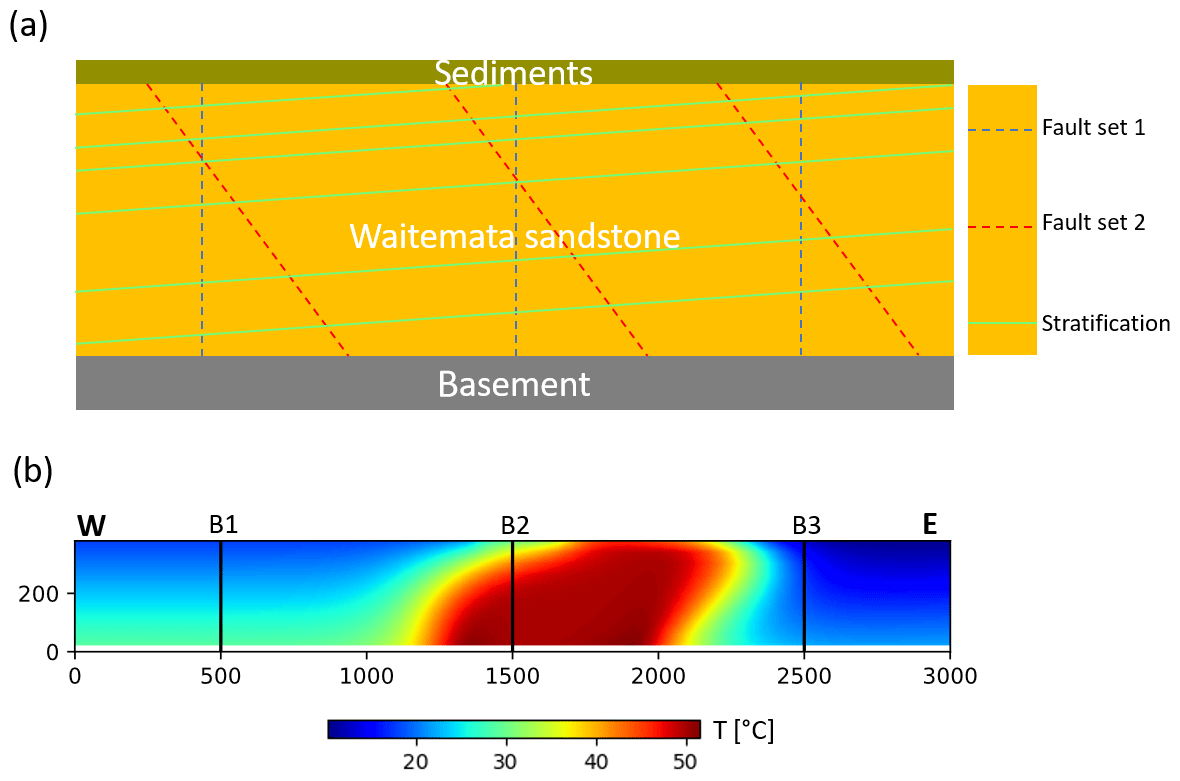
Figure 1Geological and thermal conditions of the Waiwera geothermal site. (a) Structural elements of the aquifer, (b) interpolated temperature distribution.
The aquifer body is formed of the Waitemata sandstone formation, which is a strongly stratified sandstone with a hydraulic conductivity of m s−1 (average of entire setting determined by a pumping test). The spacing of the stratification is unknown (Kühn et al., 2016). The stratification is not horizontal, because the formation has been folded, fractured and faulted (Kühn and Schöne, 2017). It is also intersected by two high inclination fault sets (Fig. 1a). One of these faults provide the pathway for the geothermal water at the aquifer bottom. From hydraulic tests and well drill activities the hydraulic conductivity of faults and fractures is estimated (in the range of 10−4–10−6 m s−1) and used in the inversion (ARWB, 1987).
Previous studies modelled the aquifer using continuum approaches, combining the hydraulic properties of the fractures, the stratification and the aquifer matrix (Kühn et al., 2016; Kühn and Altmannsberger, 2016; Kühn and Stöfen, 2005). These models however do not include the discrete features and could not describe the thermo-hydraulic behavior of the aquifer. The aim of this study is to interpret the borehole temperature profiles with DFN models, to infer the geometry of the faults.
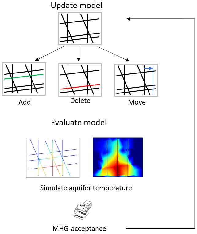
Figure 2The transdimensional DFN inversion algorithm. Every iteration of the inversion consists of two phases. In the model update phase, the DFN is modified randomly, via fracture deletion, addition or horizontal translation of a fault. In the model evaluation phase, the updated model is evaluated by simulating the temperature field in the aquifer.
3.1 Inversion
In this study we use the transdimensional DFN inversion introduced by (Somogyvári et al., 2017), based on the reversible-jump Markov chain Monte Carlo (rjMCMC) algorithm (Green, 1995). This iterative technique uses subsequent random geometry perturbations to generate and test possible model configurations (Fig. 2). Every iteration consists of two phases: an update and an evaluation phase.
In the update phase, the current DFN realization (θn) is altered by fracture addition, deletion or movement. The type of the update and its properties are chosen randomly, with a predefined probability (). Fractures could only be inserted to specific discrete points along the existing DFN. This is an important condition to preserve the reversibility of the chain (see Somogyvári et al., 2017).
In the evaluation phase the temperature distribution in the aquifer is modelled on the updated DFN realization (θ∗) using the forward model (details in Sect. 3.2). The model evaluation is done using the Metropolis-Hastings-Green acceptance criterion (Green, 1995):
The likelihood-ratio () is calculated from the improvement of the RMS error of the simulated observations (ξ|θ). We consider the observations (ξ) normally distributed, hence the L functions have a gaussian shape. The proposal ratio () is calculated as the ratio of the probabilities of the reverse and the forward update. Because these updates are discrete, the calculation of these probabilities are straightforward. For example, the probability of a fracture deletion is one over the total number of fractures. A detailed description on the update probabilities can be found in (Somogyvári et al., 2017). The so-called Jacobian (|J|) is a consequence of the transdimensional updates, and it is required to maintain the stability of the rjMCMC. With discrete model updates however, its value is always one (Denison et al., 2002).
If a proposal gets accepted the new iteration starts with it, if it gets rejected the chain continues with the previous realization. The final product of rjMCMC inversion is not one calibrated model, but a set of realizations often referred to as ensemble. The ensemble is suitable for further statistical investigations and for uncertainty analysis (Somogyvári et al., 2017). To eliminate the effect of the arbitrary chosen initial model, the first part of the chain is discarded and not used in the ensemble (Somogyvári and Reich, 2019).
3.2 Forward model
To simulate the steady state temperature distribution in the DFN model, the tracer transport simulator developed by Jalali (2013) was used. This efficient algorithm could simulate temperature distributions in two dimensional DFN models within a few seconds, making it suitable for MCMC applications.
The forward model takes the DFN geometry and hydraulic and temperature boundary conditions as an input and returns the steady state temperature distribution in the fracture network. The simulator is transient, both the pressure and temperature simulations start from an initial field with perturbations by the boundary conditions, then the simulation is run until a steady pressure and temperature field is obtained.
First the DFN model is discretized to 1-D segments and nodes. Pressure distribution is simulated by using mass conservation, with an implicit finite difference method. Flow in the fractures are calculated by Darcy's law from the pressure gradient. For thermal transport, the advection-dispersion equation is solved considering a steady-state flow field, with an implicit upwind finite difference solver (Jalali, 2013; Ringel et al., 2019).
In this simple model no temperature transport is simulated within the impermeable rock matrix, only the temperature loss from the fracture space towards the rock matrix is simulated. Hence, cross-fracture heat transport (between non-connected near fractures) is not possible. The simulation is limited to 2-D and no complex hydraulic and thermohaline boundary conditions are considered.
The temperature field inside the non-fractured aquifer matrix is calculated via linear interpolation with triangulation. The interpolated field is then intersected with the boreholes, and the extracted 1-D temperature profiles were used as the simulated observations. In theory it would be possible to compare the interpolated 2-D temperature field, with the interpolated field from the site (see Fig. 1b), but we wanted to demonstrate the robustness of the method with only using temperature logs from a limited number of boreholes. The complete simulation could be done faster than a second on a laptop, thus this simple DFN transport model is efficient and fast to be used in an MCMC framework.
3.3 Conceptual model
The methodology introduced in (Somogyvári et al., 2017) needed to be modified to work on reservoir scale scenarios. The main modification is a simplification to mitigate the limited amount of observations available. Three fracture sets are defined: two for the major fault directions and one for the stratification. In this modified setting, fractures are completely intersecting the domain. This simplification is done based on the geological model of the aquifer (Fig. 1a). Hence, fracture lengths are not a free parameter of the inversion as they are calculated from the fracture position within the domain. In addition, fracture centers are aligned to the vertical or horizontal centerline of the domain (depending on the fracture set) – basically reducing the free parameters to one per fracture.
Some further modifications were also done. Fracture addition and deletion is only used for the low-inclination fracture set (stratification), and fracture movement only for the high inclination sets (the exact location of these faults is not known).
The hydraulic and thermal fracture properties were chosen after available borehole information. The two fault sets are simulated with an aperture of 0.5 mm. The stratification aperture is set to 0.8 mm. These values are chosen after (Kühn et al., 2016) using the cubic law to convert transmissivities to apertures. The values were further tuned by preliminary modelling trying to obtain similar extent of the temperature anomaly as the observed one. These tests also showed that the anisotropy has a stronger effect than the exact aperture values. The hydraulic conductivities of the fractures are calculated from the apertures using the cubic law. Note that both flow and heat transport is limited to 2-D in the model, and no 3-D effects are considered.
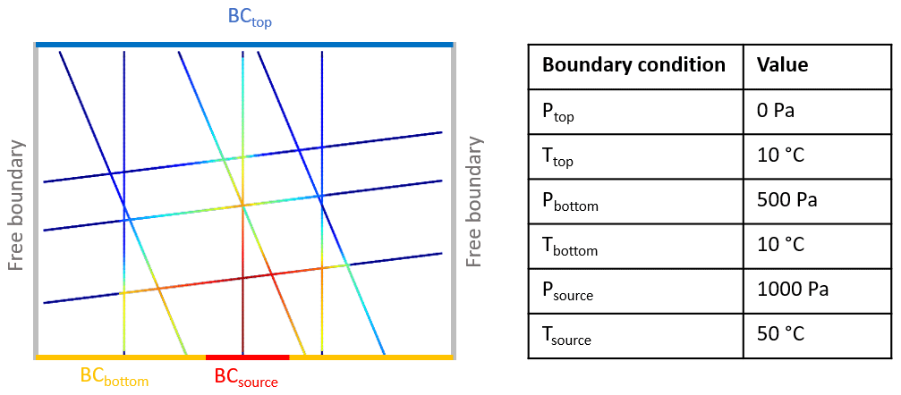
Boundary conditions are defined on the top and bottom borders (Fig. 3). In the DFN forward models, they appear when a fracture intersects with these borders. Note that the used pressure values are not absolute and were selected after the hydraulic gradient. For the source of the geothermal water, a 100 m long source region with increased pressure and temperature is defined in the bottom center of the model. The observed maximum temperature of 50 ∘C was assigned. Pressure of the source region was arbitrarily selected after the parameter tests with inspecting the extent of the temperature anomaly (Fig. 3).
Note that the used methodology is limited to invert the geometry, and does not estimate the physical fracture properties. Introducing the hydraulic parameters of the fractures as free parameters into the inversion would result in an increase in model freedom, which without involving additional data would lead to different equivalent solutions (Somogyvári et al., 2017).
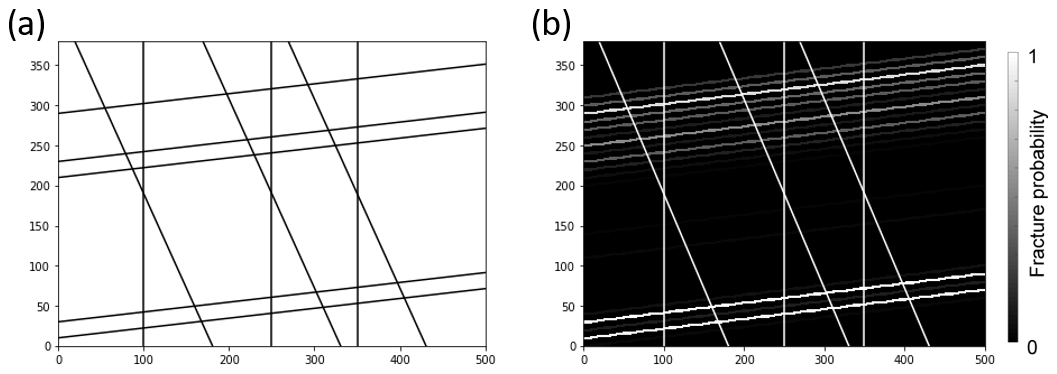
Figure 4Reconstruction of the synthetic DFN example: (a) Synthetic DFN model, (b) Reconstructed fracture probability map.
4.1 Synthetic modelling
The method was first tested on a synthetic dataset. The chosen synthetic DFN model is shown in Fig. 4a. The inversion here is limited to the fractures representing the stratification. The high inclination faults are considered known, and not estimated by the algorithm.
The transdimensional DFN inversion was implemented in python and was run on a standard office laptop with an Intel i5-7267U CPU. The chains were run for 1000 iterations which took 5 min on average. Because of the stochastic nature of the used inversion technique, we ran several simulations with the same initial parameters to see the stability of the results. All these simulations led to reconstructed geometries with the same general features, showing the robustness of the algorithm.
The result of the synthetic example is shown in Fig. 4b in the form of a fracture probability map. This plot visualizes the realizations of the rjMCMC chain by rasterizing the DFN models first, then counting the pixels with fractures along the ensemble. This is equivalent of taking the mean of the MCMC chain for visualization (Bodin and Sambridge, 2009). The fracture probability map shows perfect fits with the two fractures in the bottom part of the profile. The three fractures in the top are not captured exactly, but the extension of this fractured zone is well resolved. The absence of fractures in the center part is captured perfectly. This result is a proof of concept that the methodology is applicable on the proposed geological problem.
4.2 Field modelling
For field application, the three virtual boreholes defined as 1-D slices of the profile shown in Fig. 1b were chosen. One borehole is taken from the center of the anomaly, the other two from the two sides. These virtual boreholes were selected instead of real wells for practical reasons, as all temperature profiles from the site were already compiled and integrated to a 3-D temperature dataset. This removes any local effects of the actual boreholes and also provide room for sensitivity analysis of different borehole locations numbers along the profile, which is to be done in the future.
To improve the estimation, background temperature trends were removed from the virtual boreholes (using the temperature trends from the two sides of the model). With the removal of these trends, we have also mitigated the effect of freshwater-seawater mixing, which is not simulated by the forward model.
Simulations were run for 1000 iterations, and similarly to the synthetic case the first half of the chain was discarded. The simulations were completed within 15 min, a little longer then the synthetic case. The results are presented in Fig. 5.
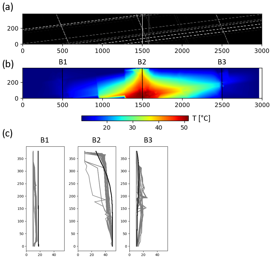
Figure 5(a) Fracture probability map of the Waiwera geothermal aquifer, (b) mean temperature field of the reconstructions (c) observed borehole temperature profiles (black) and reconstructed borehole profiles (gray).
The reconstructed fracture probability map has the following three distinct features. Strong stratification is present close to the bedrock with high probability. Fractures in this area are close to the source and provide pathways for the heat to spread out horizontally. A non-stratified aquifer body present in the center of the domain. It could not only mean that this part is non-fractured, this could be also explained with the existence of fractures that do not play a role of forming the anomaly. This is supported by the similarity of additional synthetic examples where this feature was usually present. In contrast, there is high probability of stratification in the top. The role of these fractures is to close the anomaly, by allowing mixing with the colder waters. The inversion also placed faults close to the location of two boreholes for similar reasons.
Figure 5b shows the mean of the reconstructed temperature fields of the ensemble. Compared to the observed temperature anomaly, the reconstruction shows similar properties. The two anomalies have a comparable extent horizontally and vertically. The skewedness of the anomaly is reconstructed. Originally this was explained by the mixing of different waters, but our results show that it could be explained by the structure of the aquifer.
Figure 5c shows the fit quality of the borehole temperature profiles. Continuous models from the same site provide better fits for most of the temperature observations (Kühn and Stöfen, 2005) but cannot match some observations which are supposed to be based on the fractured characteristic of the reservoir rock. The main limitations here are the 2-D simulation and the lack of complex geometry options, which restricts the shape of the reconstructed anomaly. This could be addressed by generating and testing more complex fracture patterns, but can only be executed by involving additional data into the inversion.
Temperature observations are usually considered as complementary information for thecharacterization of aquifer structure (Bravo, 2002; Klepikova et al., 2014; Leaf et al., 2012). In this paper we have presented a methodology that treats steady-state borehole temperature observations as the main driver of the interpretation process. We have shown that a handful of these profiles could provide enough information to resolve the main structural elements of the investigated aquifer using a DFN based transdimensional inversion.
We used the inversion algorithm introduced by Somogyvári et al. (2017) which provides a data driven approach by keeping the number of the modelled fractures flexible throughout the inversion. The DFN model is highly conceptualized and suitable for solving the ill-posed inversion problem, given the limited amount of observations.
Using synthetic models, we have proven that the transdimensional DFN inversion, which was originally developed for tomographic observations, could be used in this significantly different scenario.
We also present the first field application of the methodology, for the characterization of the well-studied Waiwera geothermal reservoir. Transdimensional DFN inversion indicated possible locations of strongly stratified aquifer parts, and areas which are less likely to be fractured. These findings are to be validated by future explorational campaigns whose results will be also used to infer DFN models with more complexity.
Compared to other interpretations from the site using three dimensional porous medium models, the shape of the reconstructed anomaly, and the fit of the temperature profiles are less accurate. The simplified DFN model does not consider flow and transport in the rock matrix, it does not take into account the complex hydraulic and thermohaline conditions and it is also limited to two dimensions. Still despite these limitations it indicated discrete aquifer features which the continuum modelling was not capable to capture. Thus, for a complete aquifer characterization campaign, we recommend combining the two approaches, by enhancing the three-dimensional continuous models by the discrete features obtained from DFN modelling.
We did not explore the stochastic behavior of the methodology, the resulted ensemble could be the subject of further statistical analysis and uncertainty quantification (Somogyvári et al., 2017; Somogyvári and Reich, 2019). This aspect will be investigated in a future study. The presented interpretations are to be used to select aquifer sections for more detailed exploration, to characterize the hydraulic properties of the fractures and identify the locations of the faults.
The data of this study is not openly available, but it can be provided upon request by the corresponding author.
The analysis of the data and the preparation of the scripts were performed by MS. The data was provided and prepared by MK. SR assisted with the methodology development. The manuscript was prepared by MS.
The authors declare that they have no conflict of interest.
This article is part of the special issue “European Geosciences Union General Assembly 2019, EGU Division Energy, Resources & Environment (ERE)”. It is a result of the EGU General Assembly 2019, Vienna, Austria, 7–12 April 2019.
This research has been supported by the Geo.X, the Research Network for Geosciences in Berlin and Potsdam (grant no. SO_087_GeoX) and the Deutsche Forschungsgemeinschaft (DFG) (grant no. CRC 1294 “Data Assimilation (Project B04)).
This open-access publication was funded
by Technische Universität Berlin.
This paper was edited by Thomas Nagel and reviewed by four anonymous referees.
ARWB: Waiwera water resource survey – Preliminary water allocation/management plan, Auckl. Reg. Water Board, Tech. Publ., 17, 1980.
ARWB: Waiwera thermal groundwater allocation and management plan 1986, Auckl. Reg. Water Board, Tech. Publ., 39, 1987.
Bodin, T. and Sambridge, M.: Seismic tomography with the reversible jump algorithm, Geophys. J. Int., 178, 1411–1436, https://doi.org/10.1111/j.1365-246X.2009.04226.x, 2009.
Bravo, H. R.: Using groundwater temperature data to constrain parameter estimation in a groundwater flow model of a wetland system, Water Resour. Res., 38, 28-1–28-14, https://doi.org/10.1029/2000WR000172, 2002.
Day-Lewis, F. D., Hsieh, P. A., and Gorelick, S. M.: Identifying fracture-zone geometry using simulated annealing and hydraulic-connection data, Water Resour. Res., 36, 1707–1721, https://doi.org/10.1029/2000WR900073, 2000.
Denison, D. G. T., Adams, N. M., Holmes, C. C., and Hand, D. J.: Bayesian partition modelling, Comput. Stat. Data An., 38, 475–485, https://doi.org/10.1016/S0167-9473(01)00073-1, 2002.
Dorn, C., Linde, N., Borgne, T. Le, Bour, O., and de Dreuzy, J. R.: Conditioning of stochastic 3-D fracture networks to hydrological and geophysical data, Adv. Water Resour., 62, 79–89, https://doi.org/10.1016/j.advwatres.2013.10.005, 2013.
Green, P. J.: Reversible jump Markov chain monte carlo computation and Bayesian model determination, Biometrika, 82, 711–732, https://doi.org/10.1093/biomet/82.4.711, 1995.
Hao, Y., Yeh, T.-C. J., Xiang, J., Illman, W. A., Ando, K., Hsu, K.-C., and Lee, C.-H.: Hydraulic Tomography for Detecting Fracture Zone Connectivity, Ground Water, 46, 183–192, https://doi.org/10.1111/j.1745-6584.2007.00388.x, 2008.
Hestir, K., Martel, S. J., Vail, S., Long, J., D'Onfro, P., and Rizer, W. D.: Inverse hydrologic modeling using stochastic growth algorithms, Water Resour. Res., 34, 3335–3347, https://doi.org/10.1029/98WR01549, 1998.
Hui, M.-H., Dufour, G., Vitel, S., Muron, P., Tavakoli, R., Rousset, M., Rey, A., and Mallison, B.: A Robust Embedded Discrete Fracture Modeling Workflow for Simulating Complex Processes in Field-Scale Fractured Reservoirs, in: SPE Reservoir Simulation Conference, 10–11 April 2019, Galveston, Texas, USA, 2019.
Illman, W. A. and Neuman, S. P.: Steady-state analysis of cross-hole pneumatic injection tests in unsaturated fractured tuff, J. Hydrol., 281, 36–54, https://doi.org/10.1016/S0022-1694(03)00199-9, 2003.
Illman, W. A., Liu, X., Takeuchi, S., Yeh, T.-C. J., Ando, K., and Saegusa, H.: Hydraulic tomography in fractured granite: Mizunami Underground Research site, Japan, Water Resour. Res., 45, W01406, https://doi.org/10.1029/2007WR006715, 2009.
Jalali, M.: Thermo-Hydro-Mechanical Behavior of Conductive Fractures using a Hybrid Finite Difference – Displacement Discontinuity Method, 187, available at: http://hdl.handle.net/10012/7642 (last access: 23 February 2017), 2013.
Jang, I. S., Kang, J. M., and Park, C. H.: Inverse Fracture Model Integrating Fracture Statistics and Well-testing Data, Energ. Source. Part A, 30, 1677–1688, https://doi.org/10.1080/15567030802087510, 2008.
Klepikova, M. V., Le Borgne, T., Bour, O., and de Dreuzy, J.-R.: Inverse modeling of flow tomography experiments in fractured media, Water Resour. Res., 49, 7255–7265, https://doi.org/10.1002/2013WR013722, 2013.
Klepikova, M. V., Le Borgne, T., Bour, O., Gallagher, K., Hochreutener, R., and Lavenant, N.: Passive temperature tomography experiments to characterize transmissivity and connectivity of preferential flow paths in fractured media, J. Hydrol., 512, 549–562, https://doi.org/10.1016/j.jhydrol.2014.03.018, 2014.
Kühn, M. and Altmannsberger, C.: Assessment of Data Driven and Process Based Water Management Tools for the Geothermal Reservoir Waiwera (New Zealand), Energy Proced., 97, 403–410, https://doi.org/10.1016/j.egypro.2016.10.034, 2016.
Kühn, M. and Schöne, T.: Multivariate regression model from water level and production rate time series for the geothermal reservoir Waiwera (New Zealand), Energy Proced., 125, 571–579, https://doi.org/10.1016/j.egypro.2017.08.196, 2017.
Kühn, M. and Stöfen, H.: A reactive flow model of the geothermal reservoir Waiwera, New Zealand, Hydrogeol. J., 13, 606–626, https://doi.org/10.1007/s10040-004-0377-6, 2005.
Kühn, M., Altmannsberger, C., and Hens, C.: Waiweras Warmwasserreservoir – Welche Aussagekraft haben Modelle?, Grundwasser, 21, 107–117, https://doi.org/10.1007/s00767-016-0323-2, 2016.
Leaf, A. T., Hart, D. J., and Bahr, J. M.: Active Thermal Tracer Tests for Improved Hydrostratigraphic Characterization, Ground Water, 50, 726–735, https://doi.org/10.1111/j.1745-6584.2012.00913.x, 2012.
Le Borgne, T., Bour, O., Riley, M. S., Gouze, P., Pezard, P. A., Belghoul, A., Lods, G., Le Provost, R., Greswell, R. B., Ellis, P. A., Isakov, E., and Last, B. J.: Comparison of alternative methodologies for identifying and characterizing preferential flow paths in heterogeneous aquifers, J. Hydrol., 345, 134–148, https://doi.org/10.1016/j.jhydrol.2007.07.007, 2007.
Le Goc, R., de Dreuzy, J.-R., and Davy, P.: An inverse problem methodology to identify flow channels in fractured media using synthetic steady-state head and geometrical data, Adv. Water Resour., 33, 782–800, https://doi.org/10.1016/j.advwatres.2010.04.011, 2010.
Long, J. C. S., Remer, J. S., Wilson, C. R., and Witherspoon, P. A.: Porous media equivalents for networks of discontinuous fractures, Water Resour. Res., 18, 645–658, https://doi.org/10.1029/WR018i003p00645, 1982.
Neuman, S. P.: Trends, prospects and challenges in quantifying flow and transport through fractured rocks, Hydrogeol. J., 13, 124–147, https://doi.org/10.1007/s10040-004-0397-2, 2005.
Niven, E. B. and Deutsch, C. V.: Non-random Discrete Fracture Network Modeling, in: Quantitative Geology and Geostatistics, 17, edited by: Abrahamsen, P., Hauge, R., and Kolbjørnsen, O., 275–286, Springer Netherlands, Dordrecht, 2012.
Pan, Y., Hui, M.-H., Narr, W., King, G. R., Tankersley, T., Jenkins, S., Flodin, E., Bateman, P., Laidlaw, C., and Vo, H. X.: Integration of Pressure-Transient Data in Modeling Tengiz Field, Kazakhstan – A New Way To Characterize Fractured Reservoirs, SPE Reserv. Eval. Eng., 19, 5–17, 2016.
Ringel, L. M., Somogyvári, M., Jalali, M., and Bayer, P.: Comparison of hydraulic and tracer tomography for discrete fracture network inversion, Geosci., 9, 274, https://doi.org/10.3390/geosciences9060274, 2019.
Sahimi, M.: Flow and transport in porous media and fractured rock: from classical methods to modern approaches, John Wiley & Sons., 2011.
Somogyvári, M. and Reich, S.: Convergence Tests for Transdimensional Markov Chains in Geoscience Imaging, Math. Geosci., 1–18, https://doi.org/10.1007/s11004-019-09811-x, 2019.
Somogyvári, M., Jalali, M., Jimenez Parras, S., and Bayer, P.: Synthetic fracture network characterization with transdimensional inversion, Water Resour. Res., 53, 5104–5123, https://doi.org/10.1002/2016WR020293, 2017.
Vesselinov, V. V, Neuman, S. P., and Illman, W. A.: Three-dimensional numerical inversion of pneumatic cross-hole tests in unsaturated fractured tuff: 1. Methodology and borehole effects, Water Resour. Res., 37, 3001–3017, https://doi.org/10.1029/2000WR000133, 2001.
Yao, M., Chang, H., Li, X., and Zhang, D.: Tuning Fractures With Dynamic Data, Water Resour. Res., 54, 680–707, https://doi.org/10.1002/2017WR022019, 2018.
Zha, Y., Yeh, T.-C. J., Illman, W. A., Tanaka, T., Bruines, P., Onoe, H., and Saegusa, H.: What does hydraulic tomography tell us about fractured geological media? A field study and synthetic experiments, J. Hydrol., 531, 17–30, https://doi.org/10.1016/j.jhydrol.2015.06.013, 2015.