 | 24 Sep 2019
Characterization of dredged sediments: a first guide to define potentially valuable compounds – the case of Malmfjärden Bay, Sweden
Yahya Jani
Ling Gao
William Hogland
Millions of tons of bottom sediments are dredged annually all over the world. Ports and bays need to extract the sediments to guarantee the navigation levels or remediate the aquatic ecosystem. The removed material is commonly disposed of in open oceans or landfills. These disposal methods are not in line with circular-economy goals and additionally are unsuitable due to their legal and environmental compatibility. Recovery of valuables represents a way to eliminate dumping and contributes towards the sustainable extraction of secondary raw materials. Nevertheless, the recovery varies on a case-by-case basis and depends on the sediment components. Therefore, the first step is to analyse and identify the sediment composition and properties. Malmfjärden is a shallow semi-enclosed bay located in Kalmar, Sweden. Dredging of sediments is required to recuperate the water level. This study focuses on characterizing the sediments, pore water and surface water from the bay to uncover possible sediment recovery paths and define the baseline of contamination in the water body. The results showed that the bay had high amounts of nitrogen (170–450 µg L−1), leading to eutrophication problems. The sediments mainly comprised small size particle material (silt, clay and sand proportions of 62 %–79 %, 14 %–20 %, 7 %–17 %, respectively) and had a medium–high level of nitrogen (7400–11 000 mg kg−1). Additionally, the sediments had little presence of organic pollutants and low–medium concentration of metals or metalloids. The characterization of the sediments displays a potential use in less sensitive lands such as in industrial and commercial areas where the sediments can be employed as construction material or as plant-growing substrate (for ornamental gardens or vegetation beside roads).


Ports, lakes and semi-enclosed water bodies require continuous dredging of bottom sediments to guarantee proper navigation levels and preserving the aquatic ecosystem (DelValls et al., 2004). Therefore, millions of tons of dredged sediments are generated around the world (Mymrin et al., 2017). Europe alone produces 200×106 m3 of sediments per year (SedNet, 2004). The extracted sediments are classically regarded as waste and either landfilled or disposed of in open oceans (Ali et al., 2014). However, environmental and legal reasons constrain these sediment management methods. Open ocean disposal affects the marine ecosystem, and therefore, several countries have already banned this action (Cesar et al., 2014); landfilling has long been responsible for spreading greenhouse gases and contaminated leachates, leading to different environmental impacts. Additionally, landfills are also classified as unsustainable paths of wastes since they lack the recuperation of resources and are restricted due to high space requirements (Depountis et al., 2009).
The recycling of dredged sediments in beneficial uses could be a promising route compared to the traditional disposal methods (Baxter et al., 2004). The recovery of valuables, like sediments as secondary raw materials, may contribute towards achieving sustainable circular economies. However, minimum attention has been given to developing and implementing methods for recycling or recovering dredged sediments. Recycling options may include the use in construction industries, habitat creation, plant-growing media, or the creation of dykes and covering landfills (Jani et al., 2019). In all uses, sediments can be employed as a replacement of natural raw material addressing the depletion of the Earth resources.
Recycling of dredged sediments varies on a case-by-case basis and depends on the sediment composition and physicochemical properties. Defining the composition as well as characterizing the physicochemical properties of the dredged sediments is therefore regarded as an essential step towards identifying the future route of sediments (Couvidat et al., 2018). Analysing the trace elements and organic-matter contents, nutrients and organic compounds is essential to identify potential end users and whether any prior treatment is needed (Mattei et al., 2016). High organic-matter content, nitrogen and phosphorus are essential for using the sediments in agriculture (Dang et al., 2013). However, high organic-matter content also limits the use of sediments in the construction industry due to the reduction in the durability of final products. Identifying the particle size distribution gives an essential understanding of the type of sediments and the amount of sand, silt and clay. Sandy sediments are easy to recover by separating the sand and using it in construction projects (Siham et al., 2008). Fine-grain sediments are more associated with contamination since clay and silt is bound with pollutants, and commonly chemical or biological treatment is required prior to using dredged sediments (Yoo et al., 2013).
Analysing the pore water extracted from sediments can also define the occurrence of pollutants and other components in sediments (Hammond, 2019). Additionally, characterizing sediments and surface water creates a baseline of current contamination level in a water body. Some water quality parameters are the concentration of nutrients, chlorophyll, turbidity, electrical conductivity, pH and dissolved oxygen (WHO, 1996). The status quo is vital to defining quality objectives and creating monitoring plans (Hartwell et al., 2019; Zhang et al., 2019).
This study focuses on characterizing the sediments, pore water and surface water from Malmfjärden Bay located in Kalmar, southeastern Sweden, to determine possible sediment recovery paths and define the baseline of contamination in the water body.
2.1 Site description
Malmfjärden is a semi-enclosed bay located in the city centre of Kalmar, southeastern Sweden, with minor connections to the Baltic Sea and the Western Gotland basin (Fig. 1). The bay has a special value for the municipality due to its central location which provides significant landscape and ecosystem services such as a habitat for wild birds and recreational space for inhabitants and visitors of the city. Currently, the water body is shallow, and there is a need to dredge bottom sediments to recover the normal water level to allow activities such as swimming, canoeing and wildlife development. Moreover, around the bay, there are residential and commercial areas rather than industrial sites. The bay lacks domestic and industrial sewage discharges and only receives runoff inputs. There are no published studies concerning the nutrient content and physicochemical characterization of the sediments.
2.2 Sample collection and processing
2.2.1 Sediment sampling and preparation
Sediments samples were collected from four areas in the bay to cover all the shallow region of the water body properly. The sampling area was also defined according to plans of Kalmar municipality to dredge the bay. The sampling areas covered the area that will be subject to intervention in the future. Each area contained several sampling stations. Figure 1 shows the location of the study and the sampling areas in the bay. In all stations, triplicates were collected using a manual core sampler. Sediment cores (total height of around 60 cm) were divided into top (0–20 cm) and bottom (20–60 cm) layers to identify a possible differences in their composition. The layers were separated using a plastic spatula, and composite samples of each of the four groups were created by manually mixing the sediments using pre-cleaned polyethene bags. Samples were stored in pre-cleaned polyethene bags at 4 ∘ C before laboratory analyses.
2.2.2 Pore water preparation
Pore water was extracted following the procedure used by Charbonnier et al. (2019). The sediments were centrifuged in a Beckman Avanti J-25 (USA) centrifuge at a speed of 4000 rpm for 15 min. One general sample was formed mixing the pore water extracted from each core. Only one sample, instead of several samples per group, was delivered to analysis due to the high volume requirement from the private laboratory. The extracted pore water was collected in a pre-clean acid-washed (with 15 % HCl) container and preserved at 4 ∘C before analyses.
2.2.3 Surface water sampling and preparation
Surface water samples were taken from the same sediment stations. The surface water was sampled at a depth of around 10 cm. The samples were stored in pre-cleaned acid-washed containers (rinse with 15 % HCl) at 4 ∘C before analyses.
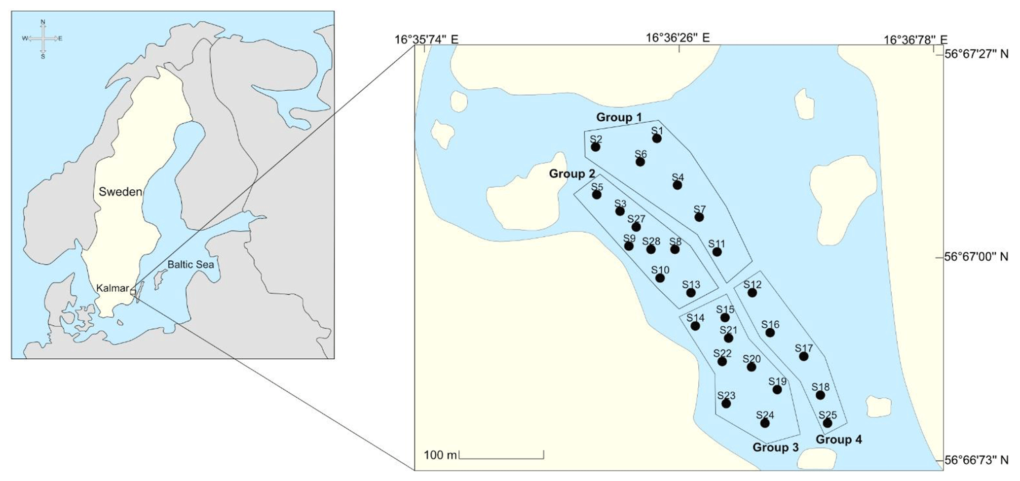
Figure 1Location of the study area and sampling stations.
2.3 Analytical methods
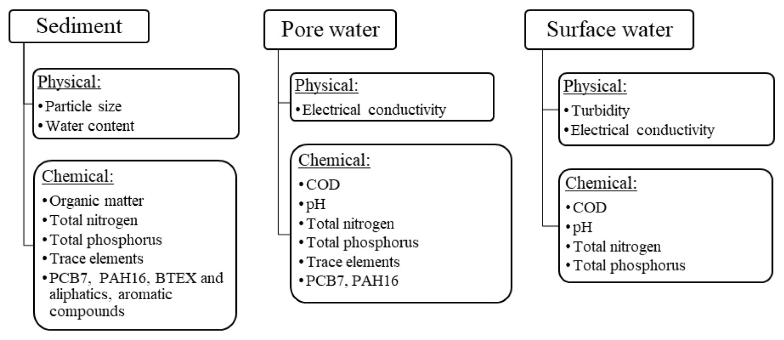
The analyses performed on sediments, pore water and surface water are shown in Fig. 2. The analytical methods are further explained in Sect. 2.3.1 and 2.3.2.
2.3.1 Physicochemical characteristics – sediments
Composite samples of top and bottom sediments from each of the four groups were employed to determine the composition of the sediments. The solid content was measured by drying 50 g of each sample in an oven at 105±5 ∘C until achieving a constant weight (EN 12880:2000). The solid content was calculated using the weight difference before and after drying. After concluding the solid content test, part of the same samples was used to calculate the organic content (loss on ignition test). Approximately 10 g of dry sediments was heated at 550 ∘C for 1 h (SS-EN 15169:2007). The organic content was calculated by finding the weight difference before and after drying. All samples were analysed in duplicates.
The chemical characteristics of the sediments were analysed at the commercial laboratory SYNLAB- Sweden. The samples were digested and processed according to EN-ISO-11885, and the elements were measured by inductively coupled plasma atomic emission spectroscopy (ICP-AES). Organic compounds were measured by gas-chromatography–mass-spectrometry (GC-MS). The total nitrogen was analysed following the Kjeldahl procedure (SS-EN 16169:2012). Samples for trace elements and nutrients were analysed in duplicates, while organic compounds were analysed without replicating it due to previous indications of low organic-pollutant levels at this site.
The sediment particle size distribution was found by the wet-sieve methodology followed by the pipette method given by Poppe et al. (2000). According to previous knowledge, the particle size distribution in the bay has a constant uniformity; therefore, only one general composite sample from the top layers and one from the bottom layers were generated to carry out the test. The accumulated particle size graph was plotted using the software DPlot version 2.3.5.7.
2.3.2 Physicochemical characteristics – water phases
Contents of trace elements and organic compounds in both pore and surface water were analysed at the commercial laboratory SYNLAB – Sweden. The trace element contents were measured using inductively coupled plasma atomic emission spectroscopy (ICP-AES) while total nitrogen was analysed following the Kjeldahl procedure (SS-EN ISO 11905-1:1997).
The pH, electrical conductivity and dissolved oxygen were analysed using the portable instrument WTW Multi 340i (Germany). The turbidity was measured using the equipment WTW Turb 550 IR (Germany). The chemical oxygen demand (COD) was analysed by the spectrophotometer HACH DR5000 with the cuvette LCI500 (low range: 0–150 mg L−1) or LCK114 (high range: 150–1000 mg L−1).
2.4 Statistics
The correlation between trace elements and organic matter was calculated to identify a possible relationship among the variables. The Pearson correlation analysis was carried out using the statistical software IBM SPSS (version 24).
2.5 Pollution indexes
The contamination factor (Cf) and geo-accumulation index (Igeo) were calculated to identify the sediment levels of contamination with trace elements. The Cf was found by calculating the ratio between each metal concentration to the background concentration level (Eq. 1 where Cs represents the concentration of the metal in sediment and Cb the background concentration). When the Cf value is < 1, there is no contamination; 1 < Cf < 3 exhibits moderate contamination; 1 < Cf < 3 denotes considerable contamination and Cf > 6 very high contamination (Hakanson, 1980). The Igeo was calculated using Eq. (2), where Cs represents the concentration of the metal in sediment and Cb the concentration of the same metal in the background. Igeo < 0 denotes unpolluted sediments, 0 < Igeo < 1 uncontaminated to moderately contaminated, 1 < Igeo < 2 moderately contaminated, 2 < Igeo < 3 moderately to strongly contaminated, 3 < Igeo < 4 strongly contaminated and Igeo > 5 extremely contaminated (Müller, 1969). For both indexes, the background concentrations were taken as the values provided for Sweden (SEPA, 2000).
3.1 Sediments
3.1.1 Physicochemical composition of sediments
Figure 3 shows the accumulated particle size distribution of the samples from top and bottom layers of sediments on a semi-log scale. The predominant fraction in both samples was fine particles ≤63 µm. The silt, clay and sand proportion was 79 %, 14 % and 7 % for top and 62 %, 20 % and 17 % for bottom layers, respectively. According to the classification for sediments provided by Burdige (2006c), the top sediments are categorized as silt and the bottom as sandy silt.
Dredged sediments are typically related to high water content. For handling, recycling or transporting sediments, the water content requires a reduction to useful levels (Ali et al., 2014). Table 1 illustrates the average water content in the top and bottom layers. The water content from top and bottom layers was between 71.9 % and 80.1 % and between 67.8 % and 71.7 %, respectively. Top layers contain a higher amount of water since they are closer to the water column. When a machine dredges the sediments, it is expected that the water content will increase up to 99 % and dewatering processes will be necessary to improve the transportation of sediments (Ali et al., 2014).
Table 1Composition of nutrients and the percentage of organic-matter and water content in sediments (mean ± SD; n=8). TS: total solids.
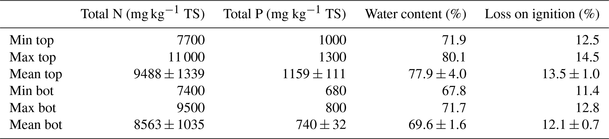
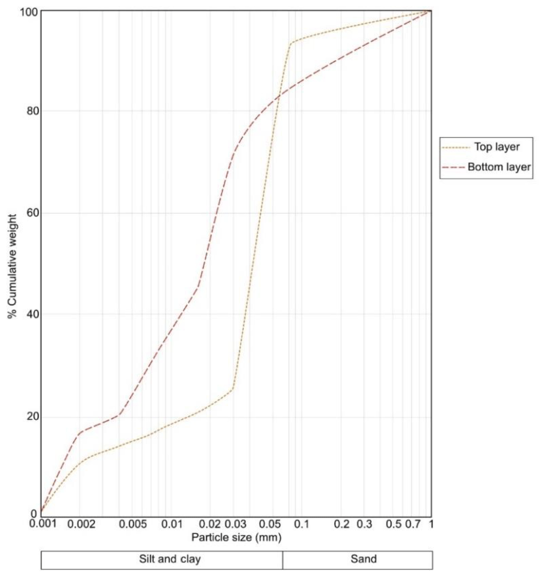
Figure 3Accumulated particle size distribution in a composite sample from top and a composite sample from bottom layers of all core sediments (semi-log scale).
Organic-matter content in sediments interacts with clay minerals to absorb or desorb anthropogenic or natural trace elements and nutrients (Ali et al., 2014). Table 1 shows the results of the organic matter of sediments represented by loss on ignition. In the study site, organic content in the top and bottom layers of sediments ranged from 12.5 % to 14.5 % and 11.4 % to 12.8 %, respectively. Both average values highlighted moderate organic content (SS-EN ISO 14688-2:2018). Results of the organic matter showed low variances between the top and bottom layers. Moreover, there is no significant difference between the two layers. The results suggested that organic matter is well distributed throughout the sediments of the sampled area of the bay.
The minimum, maximum and average concentrations of nutrients in the top and bottom layers of sediments are illustrated in Table 1. On the one hand, total phosphorus ranged from 1000 to 1300 mg kg−1 in the top and 680 to 800 mg kg−1 in the bottom layer. The concentrations in both layers have a low variance within samples from the same layer (top layer standard deviation of 10 % and bottom layer standard deviation of 5 % compared to the mean), suggesting a similar exposure to sources of phosphorus around the sampled area of the bay. However, the average concentration of phosphorus is more abundant in top than in bottom layers, possibly because of the deposition of bird faeces that highly increased the nutrient concentration in the top.
On the other hand, total nitrogen in top and bottom layers ranged from 7700 to 11 000 and 7400 to 9500 mg kg−1, respectively. In organic-rich continental sediments, the maximum concentration of nitrogen reported by Burdige (2006b) was 12 000 mg kg−1. Similar results were observed in the top and bottom layers of Malmfjärden sediments (variation of 9 %–40 %), suggesting a medium–high concentration of nitrogen. Moreover, nitrogen was significantly higher than phosphorus since the primary source of phosphorus is continental weathering and nitrogen sources include the same source as well as an atmospheric component (Burdige, 2006a).
Differences in variance in concentrations of nitrogen in top and bottom layers were insignificant (top layer standard deviation of 14 % and bottom layer standard deviation of 12 % compared to the mean). Likewise, the average concentration of the top and bottom layers was similar (difference of 10 %), suggesting that nitrogen is well distributed through the sampled area. Additionally, the sediments were always exposed to a similar nitrogen rate, probably related to the atmospheric component of the element source that provides a similar input of nitrogen over time.
Table 2Concentration of organic compounds in sediments (mean + SD; n=4). Guideline values from Swedish EPA (2009). The first value shows the maximum permissible organic-compound concentration in sensitive lands, and the second value is for less sensitive lands. Values in bold indicate components that exceed the thresholds for sensitive land.

Table 2 illustrates the concentration of target organic components in the top and bottom layers of the sampled sediments as well as their maximum permissible concentration for sensitive and less sensitive land uses (Swedish EPA, 2009). The concentration of aromatic compounds (8–10, 10–16 and 16–35), benzene, toluene, ethylbenzene, xylene (BTEX) and aliphatic compounds 5–16 were all below detection limits. The concentration of aliphatic compounds 16–35 was between 84 and 120 mg kg−1 for the top layers and between 23 and 42 mg kg−1 for the bottom layers. The concentration of polychlorinated biphenyl (PCB7) ranged from 0.73 to 12.00 and 2.80 to 4.90 µg kg−1 for the top and bottom layers, respectively. Moreover, the polycyclic aromatic hydrocarbons are introduced as follows: PAH-L, PAH-M and PAH-H for low, medium and high molecular weight, respectively. PAH-L in top layers ranged from 0.030 to 0.043 mg kg−1, and in bottom layers, all values were below the detection limit (0.03 mg kg−1). PAH-M had values between 0.57 and 1.10 and between 0.30 and 0.45 mg kg−1 for the top and bottom layers, respectively. Lastly, PAH-H ranged between 0.87 and 1.50 mg kg−1 for the top layers and between 0.38 and 0.60 mg kg−1 for the bottom layers.
The concentrations of organic components in the top and bottom layers showed insignificant variations, expressing that all the sampled area is exposed to a similar rate of pollution. However, the top presented a significantly higher concentration of aliphatic compounds 16–35. The concentrations of aliphatic compounds 16–35, PCB7, PAH-L, PAH-M and PAH-H exhibited insignificant differences between the top and bottom layers. The results suggested that organic compounds have been discharged in a similar rate except for the aliphatic compounds 16–35 that have been more abundant in recent times.
Sediments from Malmfjärden exhibited a low concentration of organic compounds. The low concentrations of these compounds can be explained by the fact that the bay has no industrial and domestic discharges and the contamination source was the runoff inputs, which is usually less polluted than sewage (Metcalf and Eddy, 2003). Regarding the Swedish guideline to determine the extent of pollution in sediments (Swedish EPA, 2009), the mean concentration of organic compounds in bottom layers met the maximum permissible concentration for sensitive lands. However, average concentrations of organic compounds in the top layer only met the less sensitive land thresholds since aliphatic compounds 16–35, PCB7 and PAH-H slightly exceeded the maximum permissible values for sensitive lands. Aliphatic compounds 16–35 and PAH-H have a higher molecular weight compared to other organic components. Therefore, they are less biodegradable and persist more in the environment. PCB7 is also a well-known persistent compound that, over time, easily prevails in the environment (Speight, 2017).
Table 3Concentration of trace elements in sediments (mean ± SD; n=8). Guideline values from Swedish EPA (2009), indicating maximum permissible metal concentration in sensitive lands and less sensitive lands. Values in bold indicate metal concentrations that exceed the guideline threshold for sensitive land.
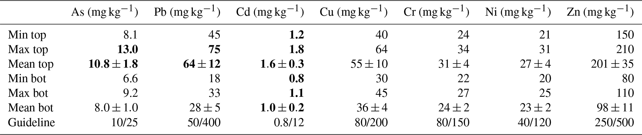
Minimum, maximum and average concentrations of trace elements from the top and bottom layers are shown in Table 3. Low variation was observed for the trace element concentration in each layer. Arsenic varied between 8.1 and 13.0 mg kg−1 in the top layer and between 6.6 and 9.2 mg kg−1 in bottom layers. Lead ranged from 45 to 75 and 18 to 33 mg kg−1 in top and bottom layers, respectively. Cadmium showed values between 1.2 and 1.8 mg kg−1 in the top layer and between 0.8 and 1.1 mg kg−1 in the bottom layer. Copper varied from 40 to 64 and 30 to 45 mg kg−1 in the top and bottom layers, respectively. Chromium ranged between 24 and 34 mg kg−1 in the top layer and between 22 and 27 mg kg−1 in the bottom layer. Nickel concentrations were valued from 21 to 31 and 20 to 25 mg kg−1 in the top and bottom layers, respectively. Lastly, zinc varied between 150 and 210 mg kg−1 in the top layer and between 80 and 110 mg kg−1 in the bottom layer.
Table 4Correlation coefficient matrix of trace elements and organic matter in sediments from the study area (n=16). LOI: loss on ignition.
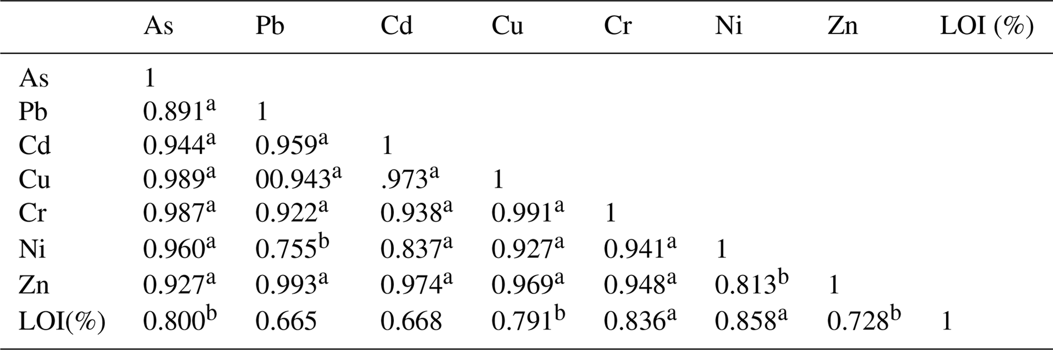
a Correlation is significant at the 0.01 level (two-tailed). b Correlation is significant at the 0.05 level (two-tailed).
On the one hand, the similar distribution of trace elements in each layer displayed that all the sampled areas were exposed to a similar rate of trace element which also suggested a common source of trace elements. The same results were confirmed by the positive correlation between average concentrations of trace elements from all sampling stations. Pearson's correlations (two-tailed) coefficients are shown in Table 4 and ranged from 0.76 to 0.99. Due to the lack of industrial and domestic sewage discharges to the study site, it is suggested that the source of trace elements could be the runoff inputs to the bay. The highest correlations were among Cu–As, Cr–As, Cr–Cu, Zn–Pb (r=0.99), implying that in the runoff these pairs of metals possibly have the same source of origin, such as vehicles emissions, residues of batteries and electrical appliances. Moreover, organic matter has a medium correlation with trace elements () which could be due to the portion of trace elements bound with organic matter. The highest correlation was between OM (organic material)–Ni (r=0.86), OM–Cr (r=0.84), OM–Cu (r=0.80), OM–As (r=0.80) and OM–Zn (r=0.73).
On the other hand, Pb, Zn, Cd and Cu displayed a major difference in average concentration between the top and bottom layers. As, Cr and Ni also revealed higher concentrations in top than in bottom layers; however, the difference was not significant. The higher concentration in top layers can be explained by the fact that, in earlier times, Kalmar had fewer vehicles, which are potentially one of the primary sources of pollution in the runoff through contaminated road dust (Hwang et al., 2016).
Sediments from Malmfjärden showed a low to medium concentration of trace elements. In top and bottom layers, Cd was the major contaminant, exceeding by 25 % the maximum permissible concentration established by the Swedish guideline for sensitive land use (Swedish EPA, 2009). As and Pb exceeded the limits for less sensitive land use by 10 % and 25 %, respectively.
3.1.2 Metal pollution indexes
Results (minimum, average and maximum) of trace element pollution indexes (Igeo and Cf) in sediments from the studied site are presented in Table 5. Both indexes denoted high contamination by cadmium. The Igeo showed moderate to low pollution by Cu, Pb, As, Zn, Ni and Cr, while the Cf illustrated moderate pollution of Pb, Cu and Zn and low contamination by As, Cr and Ni.
Table 5Pollution index for trace elements in sediments of the study area (n=16).
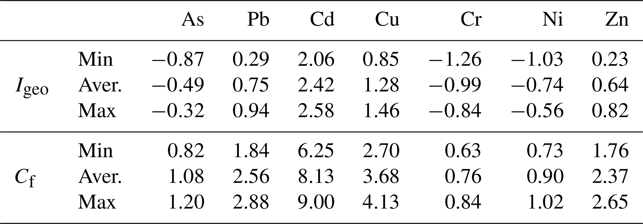
The Swedish Environmental Protection Agency estimated that sediments in Sweden have a background concentration of cadmium of approximately 0.2 ppm (Swedish EPA, 2000). The sediments from Malmfjärden presented levels of Cd around 1.3 ppm, which is 6 times higher than the background level, suggesting an anthropogenic source. Hence, it is likely that in this bay, where there are no industrial or domestic sewage discharges, the runoff may be the source of all metals including the moderate levels of Pb, Cu and Zn.
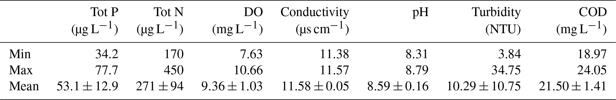
Table 6Characterization (nutrients, DO, electrical conductivity, pH, turbidity, COD) of surface water from Malmfjärden Bay (mean ± SD; n=12).
3.2 Pore water
Characterizing the properties of the pore water contributes to identifying the presence of pollutants and other components in sediments. Table 5 illustrates the concentration of trace elements, nutrients, organic pollutants and other parameters in the pore water extracted from Malmfjärden sediments. The pH was acidic (pH = 2.03), which may be due to the oxidation of iron sulfide, forming sulfuric acid when the sediments encounter atmospheric oxygen (Łukawska-Matuszewska et al., 2018). The trace element concentrations were in the order of Zn (70 µg L−1) > Pb (21 µg L−1) > As (15 µg L−1) – Cu (15 µg L−1) > Ni (8.7 µg L−1) – Cr (8.7 µg L−1) > Cd (0.64 µg L−1). It is well known that pH influences the leachability of many trace elements, and all cationic metals mainly leach out in acidic conditions (DeLaune and Smith, 1985). The low pH in the pore water could explain the low concentration of trace elements. The metalloid (As) was present at a low concentration in the pore water, presumably due to the low concentration of As in sediments that could be leached out bound with iron compounds (Banerji et al., 2019). Likewise, the pore water lacked organic pollutants (PCB7 < 0.1 ng L−1, PAH-L < 0.1 µg L−1, PAH-M < 0.2 µg L−1 and PAH-H < 0.3 µg L−1), possibly because of the low concentration of organic compounds in the sediments.
The concentration of nutrients in pore water indicated 6.7 and 14 mg L−1 of phosphorus and nitrogen, respectively. These results are in agreement with that of Łukawska-Matuszewska et al. (2018) concerning the sediments from the Baltic Sea, while the surface water showed concentrations of phosphorus and nitrogen to be around 13 and 50 times lower than that in pore water, respectively. The high concentration of nutrients in pore water is potentially related to the high concentrations of nitrogen and phosphorus in the sediments.
Lastly, chemical oxygen demand (COD) and electrical conductivity are water quality indicators. COD measures the oxygen that can be consumed by oxidizable compounds contained in water, and electrical conductivity is a measure of the water strength to transmit electrical flow, which is directly related to the amount of ions in the water (Metcalf and Eddy, 2003). Clean surface water has a COD of 20 mg L−1 and an electrical conductivity of 10 µs cm−1 (WHO, 1996). The extracted pore water from the studied sediments revealed 120 mg L−1 of COD and an electrical conductivity of 16 µs cm−1. The values showed a low electrical conductivity (low presence of ions) and medium COD, indicating the presence of compounds that can be oxidized. Due to the lack of trace elements and organic compounds in the sample, the COD is potentially associated with the nutrients in the pore water.
3.3 Surface water
Water bodies with large amounts of nutrients are classified as eutrophic. Globally, several surface water quality guidelines exist to assess eutrophication levels. The common parameters are the concentration of nutrients, dissolved oxygen, algal chlorophyll and transparency in the water. Closely, core indicators are total nitrogen and phosphorus. Table 6 shows the minimum, maximum and mean concentration of nutrients, dissolved oxygen (DO), electrical conductivity, turbidity, pH and COD. Total phosphorus varied from 34.2 to 77.7 µg L−1. Total nitrogen ranged between 170 and 450 µg L−1 and dissolved oxygen had values from 7.63 to 10.66 µg L−1. According to the Swedish guidelines for environmental quality criteria for coasts and seas (Swedish EPA, 2000), the surface water from Malmfjärden Bay showed very low levels of phosphorus, very high levels of nitrogen and high levels of dissolved oxygen. Howarth and Marino (2006) reported similar results, presenting nitrogen as one of the most substantial contamination issues for coastal waters. According to the eutrophication assessment provided by HELCOM (2018), the water body was affected by eutrophication due to the concentration of nitrogen. Andersen et al. (2011) indicated similar results for the Baltic Sea–Western Gotland basin. The turbidity in Malmfjärden ranged from 3.84 to 34.75 nephelometric turbidity units (NTU). The high variability may be due to the disturbances in the area of the bay. The mean value of turbidity was low according to the WHO guidelines values (normal values surface water: 10–100 NTU) (WHO, 1996).
The electrical conductivity of the water body ranged from 11.38 to 11.57 µs cm−1, representing minimum values reported in water bodies (typical values: 10–1000 µs cm−1) (WHO, 1996). The surface water COD ranged between 18.97 and 24.05 mg L−1 showing an average value within the range of unpolluted waters (unpolluted waters: 20 mg L−1; waters with polluted effluents: 200 mg L−1) (WHO, 1996). Lastly, the pH of surface water was between 8.31 and 8.79, representing values around the natural scale and closer to alkaline conditions (natural waters: 7–8.5). The low variance between electrical conductivity, pH and COD suggested an equal quality among the water body. According to the quality limits provided by WHO (1996), the results of electrical conductivity, turbidity, COD and pH in the surface water from Malmfjärden revealed a good-quality status in the bay.
3.4 Possible uses for sediments
Concentrations of trace elements and organic compounds in sediments from Malmfjärden only met the maximum permissible concentration for less sensitive land use. Hence, the sediments may be used directly in the construction industry or as plant-growing substrate (for ornamental gardens or vegetation beside roads) on industrial or commercial land. For construction, the high organic content influences the durability of final products, and therefore it is necessary to reduce it by thermal processes or by mixing with fly ash or other inert components (Ali et al., 2014). For plant-growing substrate, the lack of sand in the sediments suggests creating a mix of substrates (with compost, coconut fibre or peat) to improve the physical and nutrient characteristics (Mattei et al., 2018). Additionally, sediments may also be used as a final covering layer for landfills if future studies confirm the ability of sediments to create waterproof covers (Yozzo et al., 2004). All the suggested uses of sediments need to be investigated further to determine technical, environmental and economic feasibility. However, in order to reuse these sediments in sensitive lands (such as residential areas, schools and farmlands), the concentrations of cadmium in the bottom and top layers must be reduced to less than 0.8 mg L−1, while the concentrations of As, Pb, aliphatic compounds 16–35, PCB7 and PAH-H in the top layers should be reduced to less than 10, 50, 100 mg L−1, 8 µg kg−1 and 1 mg L−1, respectively.
The characterization of sediments, pore water and surface water sampled from the Malmfjärden Bay (located in southeastern Sweden) were assessed to define pollution baselines of the water body and to determine potential beneficial uses of dredged sediments. The sediment composition was dominated by silt and clay with moderate levels of organic material and a medium–high concentration of nitrogen. Organic compounds were found in low concentrations in sediments. Additionally, trace elements showed low to medium concentrations that were confirmed by the Cf and Igeo indexes denoting high contamination by cadmium and moderate pollution by Cu, Pb, As, Zn, Ni and Cr. The high correlation between the average concentration of trace elements in sediments from different sampling stations suggested that trace elements have the same source of origin. Potentially, the input of runoff may be the source of pollutants since the bay lacks industrial and domestic sewage discharges. Trace elements and organic compounds in sediments from Malmfjärden only met the maximum permissible concentration for less sensitive land use introduced by the Swedish Environmental Protection Agency (Swedish EPA, 2009). Sediments could potentially be employed for construction and as plant-growing substrate in industrial and commercial areas or as cover layers in landfills. More studies are required to verify the technical, environmental and economic feasibility.
The pore water lacked organic pollutants and had low pH values leading to low concentrations of metals or metalloids. Finally, the water body showed high concentrations of nitrogen related to eutrophication problems. However, the surface water showed levels of DO, pH, electrical conductivity, COD and turbidity in agreement with these introduce in the guidelines given by WHO (1996).
All data used were collected by the authors and are contained within this paper (see Table 1, 2, 3 and 6).
LF carried out planning, sampling, laboratory work, analysis of data and the writing of the article. YJ carried out planning, analysis of data and the writing of the article. LG carried out planning, sampling and laboratory work. WH carried out planning.
The authors declare that they have no conflict of interest.
This article is part of the special issue “European Geosciences Union General Assembly 2019, EGU Division Energy, Resources & Environment (ERE)”. It is a result of the EGU General Assembly 2019, Vienna, Austria, 7–12 April 2019.
The authors would like to thank Stefan Tobiasson and David Silfwersvärd for their contribution during the sampling campaign and Fabio Kaczala for his guidance during sampling and analysis of the results. Finally, the authors would like to state that part of the results of the study was shown at the EGU General Assembly 2019 (poster presentation).
This research has been supported by the Life Programme (grant no. LIFE15 ENV/SE/000279).
This paper was edited by Michael Kühn and reviewed by Michael Schneider and one anonymous referee.
Ali, I. B. H., Lafhaj, Z., Bouassida, M., and Said, I.: Characterization of Tunisian marine sediments in Rades and Gabes harbors, Int. J. Sediment Res., 29, 391–401, https://doi.org/10.1016/S1001-6279(14)60053-6, 2014.
Andersen, J. H., Axe, P., Backer, H., Carstensen, J., Claussen, U., Fleming-Lehtinen, V., Järvinen, M., Kaartokallio, H., Knuuttila, S., Korpinen, S., Kubiliute, A., Laamanen, M., Lysiak-Pastuszak, E., Martin, G., Murray, C., Møhlenberg, F., Nausch, G., Norkko, A., and Villnäs, A.: Getting the measure of eutrophication in the Baltic Sea: towards improved assessment principles and methods, Biogeochemistry, 106, 137–156, https://doi.org/10.1007/s10533-010-9508-4, 2011.
Banerji, T., Kalawapudi, K., Salana, S., and Vijay, R.: Review of processes controlling arsenic retention and release in soils and sediments of Bengal basin and suitable iron based technologies for its removal, Groundw. Sustain. Dev., 8, 358–367, https://doi.org/10.1016/j.gsd.2018.11.012, 2019.
Baxter, C. D. P., King, J. K., Silva, A. J., Page, M., and Calabretta, V. V.: Site Characterization of Dredged Sediments and Evaluation of Beneficial Uses, in: Proceedings of the conference Recycled Materials in Geotechnics, Baltimore, United States, 19–21 October 2004, 150–161, https://doi.org/10.1061/40756(149)10, 2004.
Burdige, D. J.: Biogeochemical Processes in Continental Margin Sediments, in: Geochemistry of Marine Sediments, Princeton University Press, United States, 97–141, 2006a.
Burdige, D. J.: An Introduction to The Organic Geochemestry of Marine Sediments, in: Geochemistry of Marine Sediments, Princeton University Press, United States, 171–217, 2006b.
Burdige, D. J.: Physical properties of sediments, in: Geochemistry of Marine Sediments, Princeton University Press, United States, 46–58, 2006c.
Cesar, A., Lia, L. R. B., Pereira, C. D. S., Santos, A. R., Cortez, F. S., Choueri, R. B., De Orte, M. R., and Rachid, B. R. F.: Environmental assessment of dredged sediment in the major Latin American seaport (Santos, Sao Paulo - Brazil): An integrated approach, Sci. Total Environ., 497, 679–687, https://doi.org/10.1016/j.scitotenv.2014.08.037, 2014.
Charbonnier, C. and Anschutz, P.: Spectrophotometric determination of manganese in acidified matrices from (pore)waters and from sequential leaching of sediments, Talanta, 195, 778–784, https://doi.org/10.1016/j.talanta.2018.12.012, 2019.
Couvidat, J., Chatain, V., Bouzahzah, H., and Benzaazoua, M.: Characterization of how contaminants arise in a dredged marine sediment and analysis of the effect of natural weathering, Sci. Total Environ., 624, 323–332, https://doi.org/10.1016/j.scitotenv.2017.12.130, 2018.
Dang, T. A., Kamali-Bernard, S., and Prince, W. A.: Design of new blended cement based on marine dredged sediment, Constr. Build Mater., 41, 602–611, https://doi.org/10.1016/j.conbuildmat.2012.11.088, 2013.
DeLaune, R. D. and Smith, C. J.: Release of Nutrients and Metals Following Oxidation of Freshwater and Saline Sediment1, J. Environ. Qual., 14, 164–168, https://doi.org/10.2134/jeq1985.00472425001400020002x, 1985.
DelValls, T. A., Andres, A., Belzunce, M. J., Buceta, J., Casado-Martinez, M. C., Castro, R., Riba, I., Viguri, J. R., and Blasco, J.: Chemical and ecotoxicological guidelines for managing disposal of dredged material, Trend. Anal. Chem., 23, 819–828, https://doi.org/10.1016/j.trac.2004.07.014, 2004.
Depountis, N., Koukis, G., and Sabatakakis, N.: Environmental problems associated with the development and operation of a lined and unlined landfill site: a case study demonstrating two landfill sites in Patra, Greece, J. Environ. Geol., 56, 1251–1258, https://doi.org/10.1007/s00254-008-1224-1, 2009.
Hakanson, L.: An ecological risk index for aquatic pollution control a sedimentological approach, Water Res., 14, 975–1001, https://doi.org/10.1016/0043-1354(80)90143-8, 1980.
Hammond, D. E.: Deep Sea Sediment: Pore Water Chemistry, in: Encyclopedia of Ocean Sciences (Third Edition), edited by: Cochran, J. K., Bokuniewicz, H. J., and Yager, P. L., Academic Press, Oxford, 82–89, 2019.
Hartwell, S. I., Dasher, D., and Lomax, T.: Characterization of metal/metalloid concentrations in fjords and bays on the Kenai Peninsula, Alaska, Environ. Monit. Assess., 191, 264, https://doi.org/10.1007/s10661-019-7376-5, 2019.
HELCOM: HELCOM Thematic assessment of eutrophication 2011–2016, Baltic Marine Environment Protection Commission – HELCOM, available at: http://www.helcom.fi/Documents/HELCOM_Thematic-assessment-of-eutrophication-2011-2016_pre-publication.pdf (last access: 15 May 2019), 2018.
Howarth, R. W. and Marino, R.: Nitrogen as the limiting nutrient for eutrophication in coastal marine ecosystems: Evolving views over three decades, Limnol. Oceanogr., 51, 364–376, https://doi.org/10.4319/lo.2006.51.1_part_2.0364, 2006.
Hwang, H.-M., Fiala, M. J., Park, D., and Wade, T. L.: Review of pollutants in urban road dust and stormwater runoff: part 1, Heavy metals released from vehicles, Int. J. Urban Sci., 20, 334–360, https://doi.org/10.1080/12265934.2016.1193041, 2016.
Jani, Y., Mutafela, R., Ferrans, L., Ling, G., Burlakovs, J., and Hogland, W.: Phytoremediation as a Promising Method for the Treatment of Contaminated Sediments, available at: http://www.ijee.net/article_85006.html (last access: 15 May 2019), Iran. J. Energy Environ., 10, 58–64, 2019.
Łukawska-Matuszewska, K. and Graca, B.: Pore water alkalinity below the permanent halocline in the Gdańsk Deep (Baltic Sea) – Concentration variability and benthic fluxes, Mar. Chem., 204, 49–61, https://doi.org/10.1016/j.marchem.2018.05.011, 2018.
Mattei, P., Cincinelli, A., Martellini, T., Natalini, R., Pascale, E., and Renella, G.: Reclamation of river dredged sediments polluted by PAHs by co-composting with green waste, Sci. Total Environ., 566–567, 567–574, https://doi.org/10.1016/j.scitotenv.2016.05.140, 2016.
Mattei, P., Gnesini, A., Gonnelli, C., Marraccini, C., Masciandaro, G., Macci, C., Doni, S., Iannelli, R., Lucchetti, S., Nicese, F. P., and Renella, G.: Phytoremediated marine sediments as suitable peat-free growing media for production of red robin photinia (Photinia x fraseri), Chemosphere, 201, 595–602, https://doi.org/10.1016/j.chemosphere.2018.02.172, 2018.
Metcalf & Eddy Inc: Chapter 2, Constituents in Wastewater, in: Wastewater engineering: treatment and reuse, Fourth edition, edited by: Tchobanoglous, G., Burton F. L., and Stensel, H. D., McGraw-Hill, Boston, 2003.
Müller, G.: Index of geoaccumulation in sediments of the Rhine River, Geojournal, 2, 108–118, 1969.
Mymrin, V., Stella, J. C., Scremim, C. B., Pan, R. C. Y., Sanches, F. G., Alekseev, K., Pedroso, D. E., Molinetti, A., and Fortini, O. M.: Utilization of sediments dredged from marine ports as a principal component of composite material, J. Clean. Prod., 142, 4041–4049, https://doi.org/10.1016/j.jclepro.2016.10.035, 2017.
Poppe, L. J., Eliason, A. H., Fredericks, J. J., Rendigs, R. R., Blackwood, D., and Polloni, C. F.: Chapter 1: Grain-size analysis of marine sediments: Methodology and data processing, in: USGS East-coast sediment analysis: Procedures, database, and georeferenced displays, United States Geological Survey, Coastal and Marine Geology Program, Woods Hole Field Center, USA, 2000.
SedNet: Contaminated Sediments in European River Basins, European Sediment Research Network, available at: https://sednet.org/wp-content/uploads/2016/03/Sednet_booklet_final_2.pdf (last accesss: 15 May 2019), the Netherlands, 2004.
Siham, K., Fabrice, B., Edine, A. N., and Patrick, D.: Marine dredged sediments as new materials resource for road construction, Waste Manage., 28, 919–928, https://doi.org/10.1016/j.wasman.2007.03.027, 2008.
Speight, J. G.: Chapter 5 – Properties of Organic Compounds, in: Environmental Organic Chemistry for Engineers, edited by: Speight, J. G., Butterworth-Heinemann, UK, 203–261, 2017.
Swedish EPA: Environmental quality criteria: Coasts and oceans, Swedish Environmental Protection Agency, Upsala, Sweden, https://www.naturvardsverket.se/Documents/publikationer/620-6034-1.pdf (last access: 15 May 2019), 2000.
Swedish EPA: Report 5976, Riktvärden för förorenad mark Swedish Environmental Protection Agency, https://www.naturvardsverket.se/Documents/publikationer/978-91-620-5976-7.pdf?pid=3574 (last access: 15 May 2019), 2009.
WHO: Water Quality Assessments – A Guide to Use of Biota, Sediments and Water in Environmental Monitoring – Second Edition, edited by: Chapman, D., E&FN Spon, available at: https://apps.who.int/iris/bitstream/handle/10665/41850/0419216006_eng.pdf;jsessionid=16A012F1475A299B9063A21DBB6912E6?sequence=1 (last access: 15 May 2019), 1996.
Yoo, J.-C., Lee, C.-D., Yang, J.-S., and Baek, K.: Extraction characteristics of heavy metals from marine sediments, Chem. Eng. J., 228, 688–699, https://doi.org/10.1016/j.cej.2013.05.029, 2013.
Yozzo, D. J., Wilber, P., and Will, R. J.: Beneficial use of dredged material for habitat creation, enhancement, and restoration in New York–New Jersey Harbor, J. Environ. Manage., 73, 39–52, https://doi.org/10.1016/j.jenvman.2004.05.008, 2004.
Zhang, H. L., Walker, T. R., Davis, E., and Ma, G. F.: Spatiotemporal characterization of metals in small craft harbour sediments in Nova Scotia, Canada, Mar. Pollut. Bull., 140, 493–502, https://doi.org/10.1016/j.marpolbul.2019.02.004, 2019.