 | 05 Jul 2019
Modelling fault reactivation with characteristic stress-drop terms
Martin Beck
Holger Class
Predicting shear failure that leads to the reactivation of faults during the injection of fluids in the subsurface is difficult since it inherently involves an enormous complexity of flow processes interacting with geomechanics. However, understanding and predicting induced seismicity is of great importance. Various approaches to modelling shear failure have been suggested recently. They are all dependent on the prediction of the pressure and stress field, which requires the solution of partial differential equations for flow and for geomechanics. Given a pressure and corresponding mechanical responses, shear slip can be detected using a failure criterion. We propose using characteristic values for stress drops occurring in a failure event as sinks in the geomechanical equation. This approach is discussed in this article and illustrated with an example.
- Article
(2161 KB) - Full-text XML
- BibTeX
- EndNote


Increased pressures in geological formations due to injection of fluids are coupled to alterations in the prevailing stress fields. In the presence of pre-existing faults, this might lead to shear failure and, as a consequence, to seismic events or earthquakes. Ellsworth (2013) defined such earthquakes as “induced” when they are triggered by human activities, no matter if the released stress is primarily caused by the activity or if it is a release of naturally existing stresses that was only triggered. He states further that earthquakes related to long-term high-volume injections, e.g. in waste-water injections, can reach magnitudes of seismic moments Mw that could lead to serious damage in buildings. There are cases reported where the epicenters where close to the injection, like in Oklahoma in 2011 with Mw=5.7 (Keranen et al., 2013) and in Texas in 2012 with Mw=4.9 (Frohlich et al., 2014), but also several kilometers away and with a time shift of 15 years as in the Paradox Valley (CO) with Mw=3.9 (Ellsworth, 2013). The question is: Why in some distance? Or why so late? It is clear that a detailed understanding of pore pressures built up by the injection and stress evolution in time and space is required, and the hydraulic and mechanical characteristics of the formation need to be considered. Very recently, the analysis of the Pohang quake in 2017, triggered by stimulation through an enhanced geothermal system, showed that magnitudes of induced quakes are not limited by the amount of injected fluid volume but can rather cause further runaway events due to complex activation of faults upon the first induced seismic event, see e.g. Lee et al. (2019).
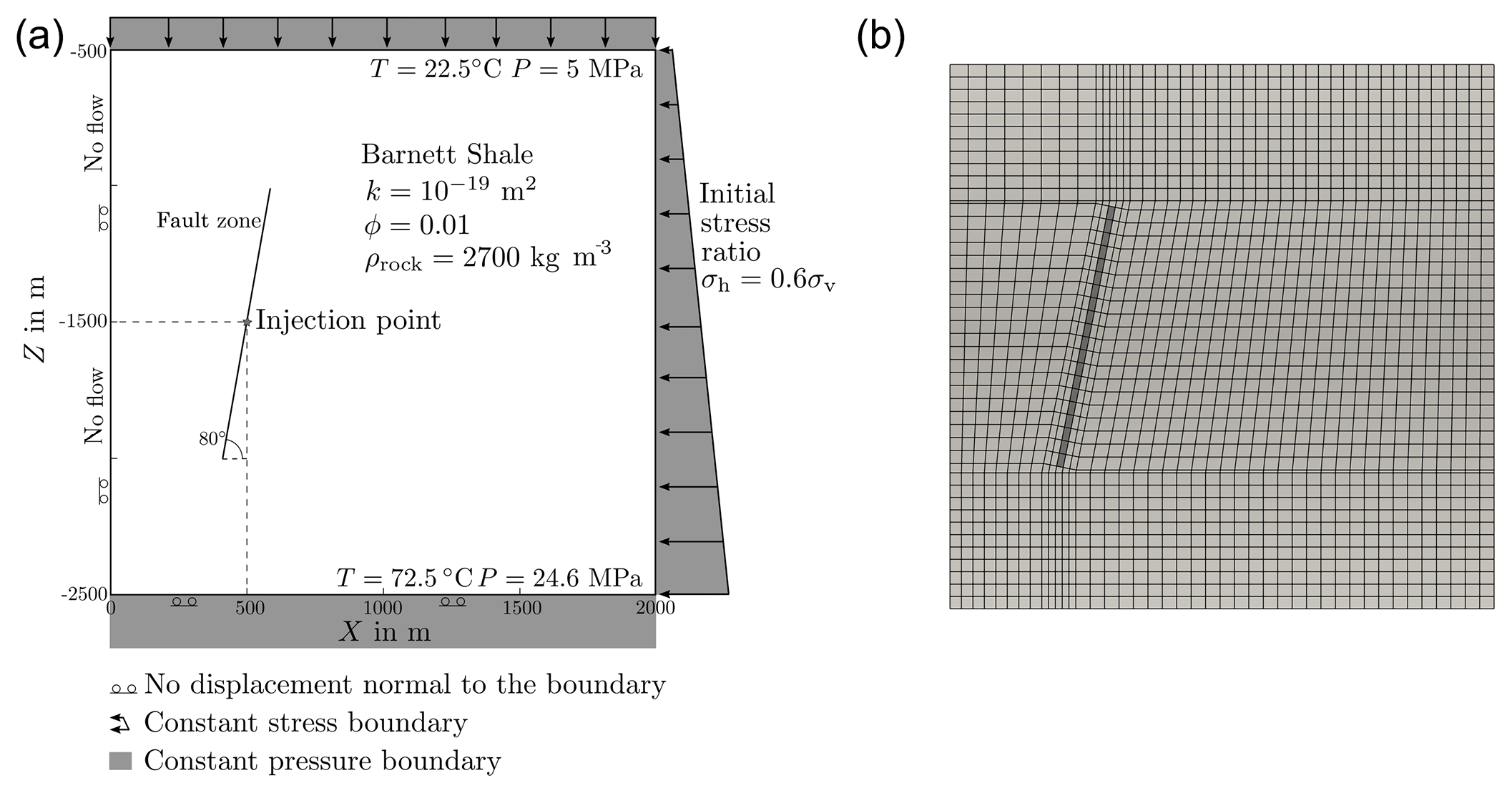
Figure 1Set-up of the hydraulic fracturing scenario after Rutqvist et al. (2013) (a) and domain discretisation (b).
Different approaches for modelling fault reactivation have been suggested. Ferronato et al. (2008) or Jha and Juanes (2014) use discrete interfaces for faults, while Cappa and Rutqvist (2011) show that describing the fault as a fault zone, and not as discrete interface, gives similar results and is less complex and less expensive.
Modelling approaches differ also in the way the physical mechanism during shear failure and seismic events is described. Current approaches use friction coefficients dependent on the slip rate and contact asperities (Jha and Juanes, 2014) or by sudden friction drops (Cappa and Rutqvist, 2011; Rutqvist et al., 2013).
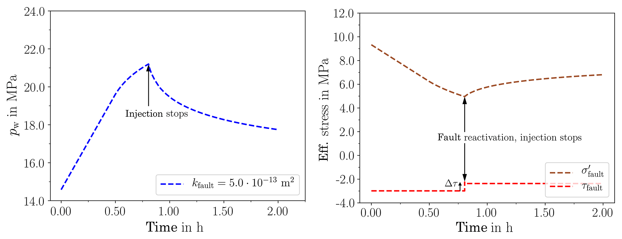
Figure 2Pressure and stress evolution (effective stress σ′ and shear stress on the fault τfault) over time at the injection cell in the fault in 1475 m depth for a fault permeability m2.
What we propose is based on energetic considerations. In a seismic event, previously built-up stress is released and transformed into seismic wave energy, heat from friction, and energy causing fracture. The shear stress is reduced on the fault plane. Accordingly, we define a stress-drop Δσfailure as the difference before and after a slip event. Literature, e.g. Aki (1972), Thatcher and Hanks (1973), Kanamori and Anderson (1975), Abercrombie and Leary (1993), reports characteristic stress drops often in a range from 0.1–1 MPa both in large and in small quakes, which is why we propose using, for example, 1 MPa as a phenomenological parameter in our model. Goertz-Allmann et al. (2011) report characteristic values larger than 2 MPa for induced seismic events at the Basel geothermal site. Therefore, the value of 1 MPa should be understood as a reasonable order of magnitude and might be adapted to other values, while it does not change the applicability of this approach for affected lengths of faults that can vary over many orders of magnitude. We claim that this is not more uncertain than complex relations with uncertain parameterisations for the friction coefficient. When, using linear elasticity, according to Mohr's circle, the pressure margin for shear failure is surpassed, the model reduces the stress at this node by a constant value of 1 MPa. The energies, into which the elastic energy is transformed, are not considered since they are either dissipated or negligible for the stress redistribution. There are other recently introduced approaches (Berge et al., 2017; Ucar et al., 2018; Gómez Castro et al., 2017) that calculate the stress drop required for reaching the equilibrium, which is in fact the excess shear stress. Our approach uses a constant value, and therefore ends up either beyond the equilibrium or does not yet reach it, the latter case would trigger immediately another failure event. What is considered more realistic depends on whether a reactivated fault stops slipping when equilibrium is reached or, due to the sudden event, goes beyond the equilibrium into a new stable state. Our model reduces the time-step size to a very small value of 0.01 s when a failure is detected, which allows resolving further events if the stress drop was not sufficient to reach a stable state.
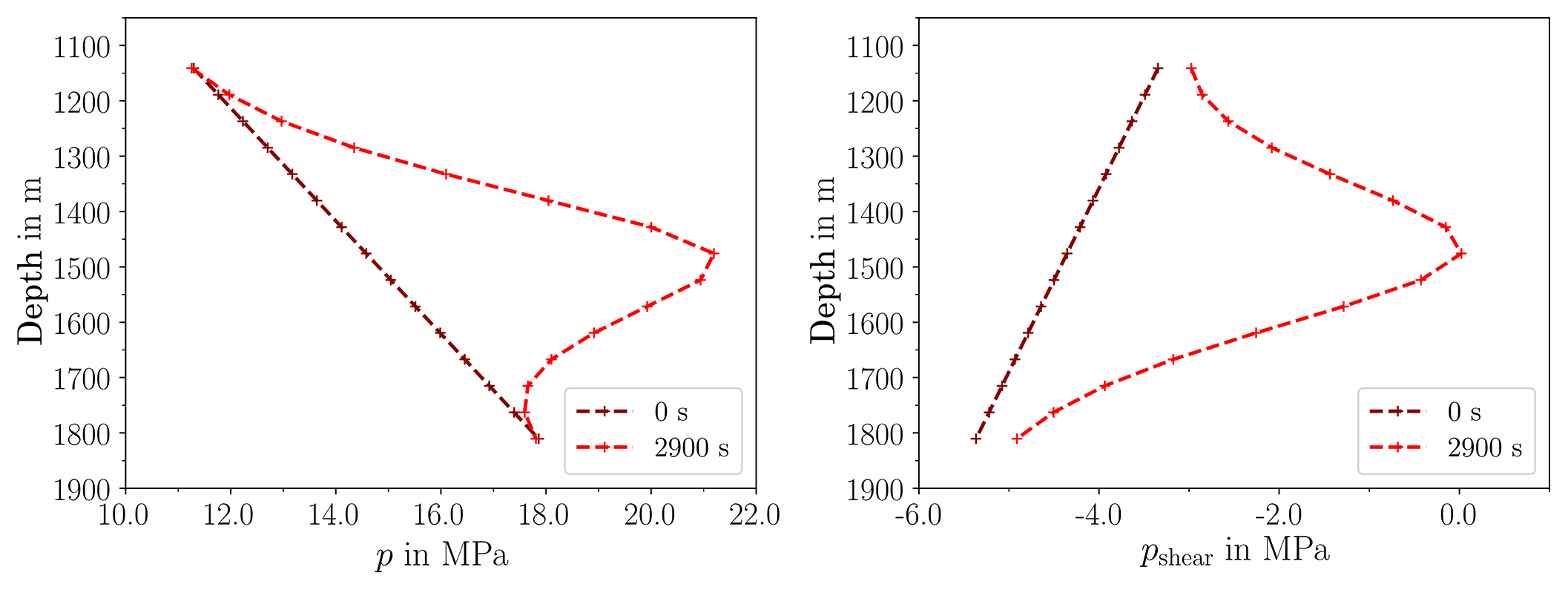
Figure 3Pressure p and pressure margin pshear for shear failure along fault at t=0 s and t=2900 s. pshear is the difference between the effective pore pressure and the critical pressure for failure.
First of all, let us very briefly review the governing equations, which are found in more detail in Beck et al. (2016), Beck (2019). Flow can be described on the “Darcy-scale” with a mass balance:
v is the Darcy velocity, ϱ fluid density. For multiphase flow, e.g. when CO2 is injected into a saline aquifer, a multiphase flow formulation with corresponding closure relations for saturations, relative permeabilities, and capillary pressures is required.
The geomechanical responses are very fast, and a quasi-steady momentum balance can be written as
with the effective stress σ′ representing the total stress reduced by the effective pore pressure (). In multiphase systems, we obtain peff as the sum of the phase pressures weighted by the saturations. α is the Biot coefficient with α=1 in the following, ϱb is the bulk density and depends on the fluid densities and the solid's density. Note that we consider only increments of stress and effective pressure relative to an initial state. We use linear elasticity to relate the stress tensor, obtained from deformations u, with the elastic properties, e.g. the bulk modulus and the shear modulus. An effective porosity is then calculated from the deformation () which can affect also permeability. The balance equations for flow and geomechanics and the corresponding closure relations are solved fully implicitly in time in a monolithic scheme, employing a quasi-staggered scheme by using the Box method for discretisation of the mass balance and a Standard Galerkin Finite Element method (both have different weighting functions!) for the momentum balance. The model is implemented in the numerical simulator Dumux (Fetzer et al., 2017).
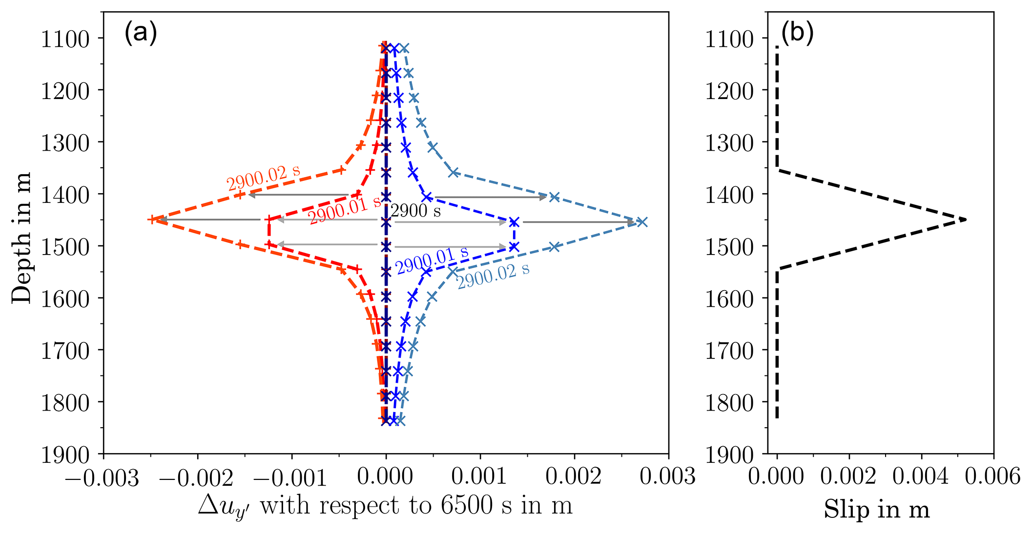
Figure 5After rotating the displacement vector into the direction of the fault: displacement in the y′-direction on the fault compared with the displacement prior to fault reactivation (a). For failed elements, the slip (b) is calculated from the difference between the displacement on the right and on the left side (grey arrows).
Pore pressures reduce compressive normal stresses and this causes a shift to the left in the Mohr circle, i.e. towards the failure curve as given by the friction coefficient. The onset of shear failure is detected when a critical pressure is reached. The fault plane can have the orientation θ of an existing fault, so the stress tensor σ can be transformed into the fault plane's direction:
Shear failure and the corresponding reduction in shear stress happens on these planes, so a predefined stress-drop value Δτ is subtracted from the shear stress:
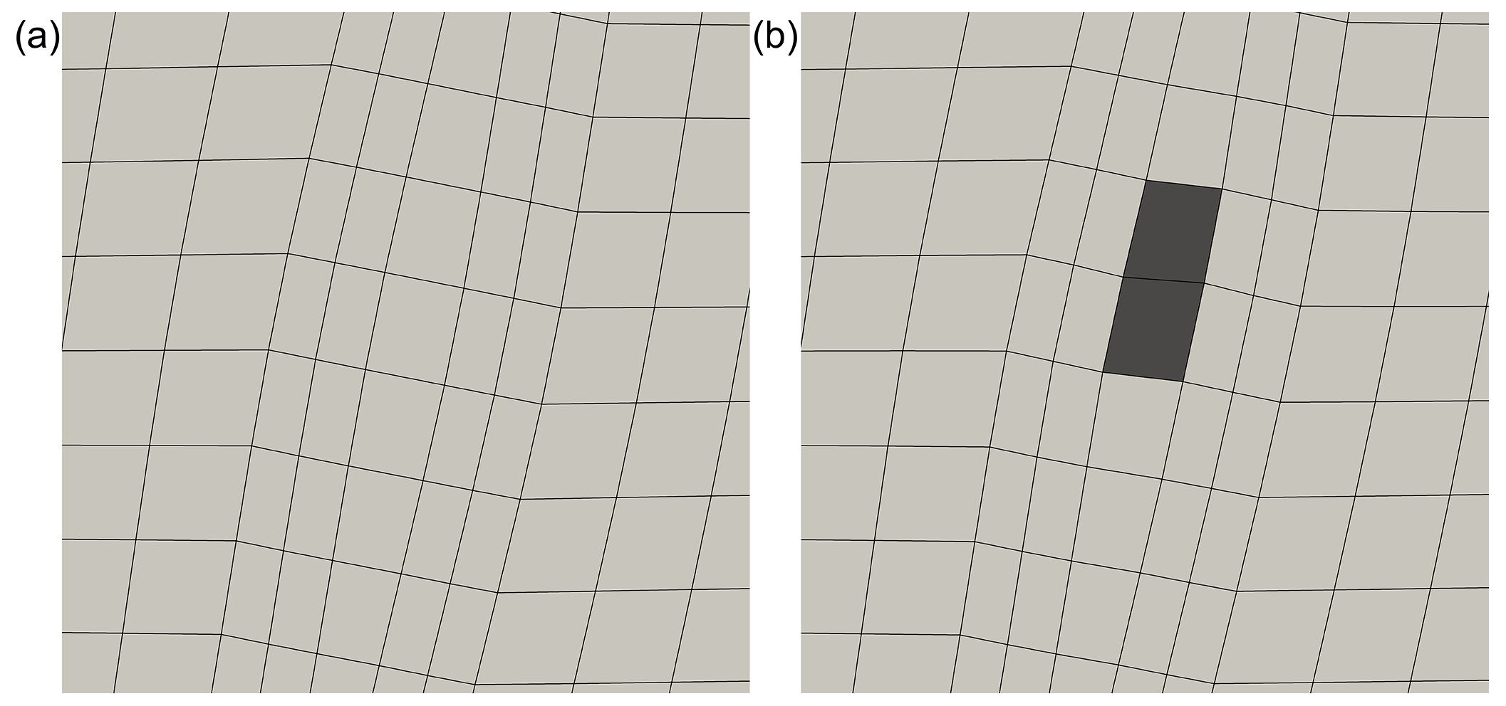
Figure 6State of deformation around the point of injection, deformations exaggerated by a factor of 1000. (a) shows the grid with only elastic deformations, (b) displays a distortion in the failed elements.
The stress tensor reduced by the stress drop is then rotated back into the original coordinates. The redistributed stresses after a stress drop on a fault plane with anisotropic variations of the local stress tensor can result in heterogeneous variation of the stress field with positive or negative impacts on other faults, coupled also to potential thermal effects as in enhanced geothermal systems, see also De Simone et al. (2017).
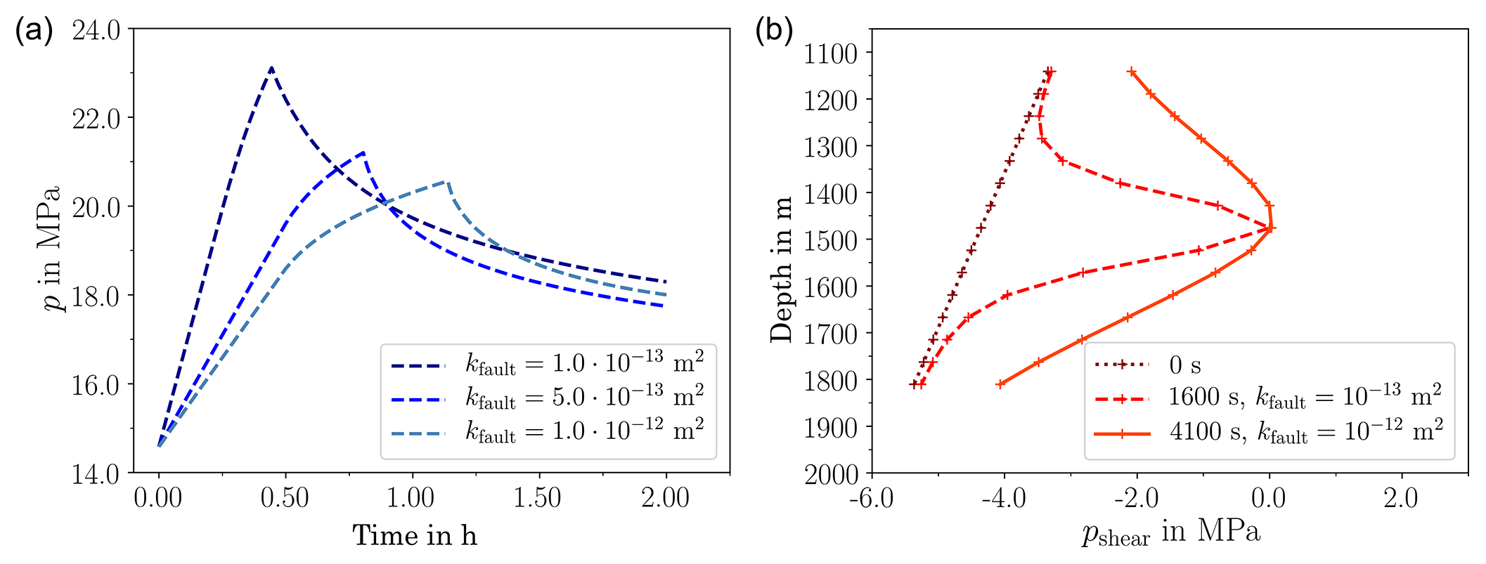
Figure 7(a) Pressure evolution over time for different fault permeabilities. (b) Distribution of the pressure margins for shear failure along the fault for different permeabilities.
The model concept proposed here slightly differs from that in our earlier publication. In Beck et al. (2016), the mechanism in the event of shear failure includes a decrease of the shear modulus in the direction of the maximum shear stress in a visco-elastic proxy model to represent a softening of the rock during the slip event. Since we formulate the momentum balance (Eq. 2) in terms of stress increments relative to an initial state, this leads at most to a reduction until zero incremental shear stress. What we propose here instead applies the constant stress drop to the total stresses, which can be dominated by the initial shear stresses. Scenarios where the main reason for shear failure is a reduction in normal stresses with almost no additional shear stress, as we will present one below, will see a significant difference in these two approaches.
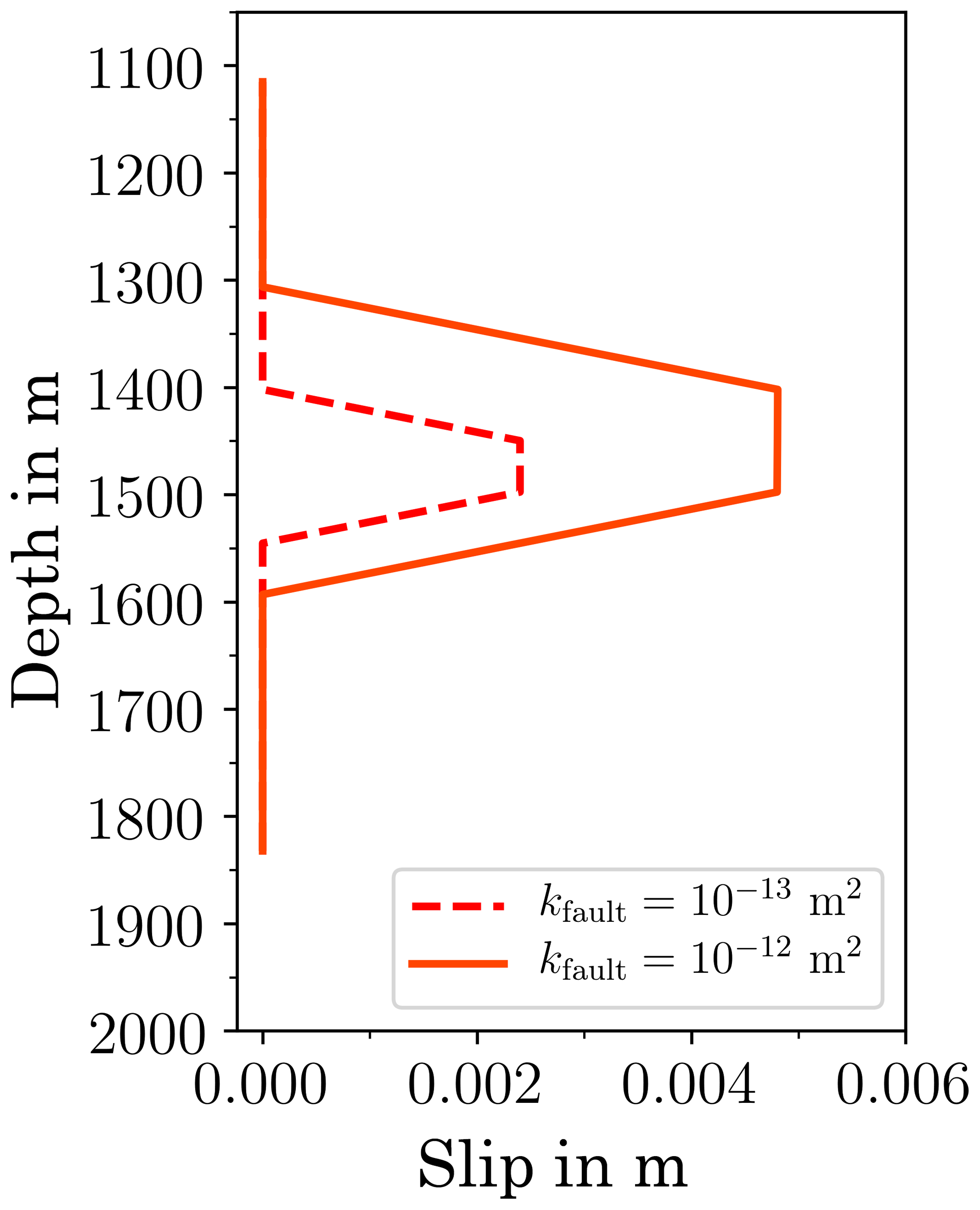
Figure 8The plot shows the resulting slip after fault reactivation for two different permeabilities. The larger slip occurs in the case with higher permeability.
The potential of injection-induced fault reactivation is illustrated using a scenario presented by Rutqvist et al. (2013) in the context of hydraulic fracturing.
3.1 Reference case
Figure 1 presents the model domain and the grid with all dimensions and boundary conditions. The setup contains a fault with the grid following its orientation. The material properties are the following (same in shale and fault if not stated otherwise): porosity ϕ=0.1, rock density ϱs=2700 kg m−3, permeability k (m2) (shale) and (fault), Young's modulus E (GPa) 30 (shale) and 5 (fault), and Poisson's ratio ν 0.2 (shale) and 0.25 (fault). No cohesion and a friction coefficient of 0.6 were assumed for the failure curve, the stress drop Δσ is 1 MPa upon a failure event. Water is injected into the fault at a rate of 0.0033 kg m−3 s−1. We chose to stop the injection when shear failure occurs.
Figure 2 shows that fault reactivation occurs after 0.75 h. In that moment, the prescribed stress drop is applied to the total stresses, which include the (in this case dominating) initial stresses, as a sink in shear stress. What happens in the details along the fault is analysed in the following.
We turn to Fig. 3. The initial pressure distribution shows an increase with depth. Over time, the pressure increases due to the injection. After 2900 s, the critical pressure for shear failure is reached in the injection element and the pressure margin exceeds the value of zero (right plot).
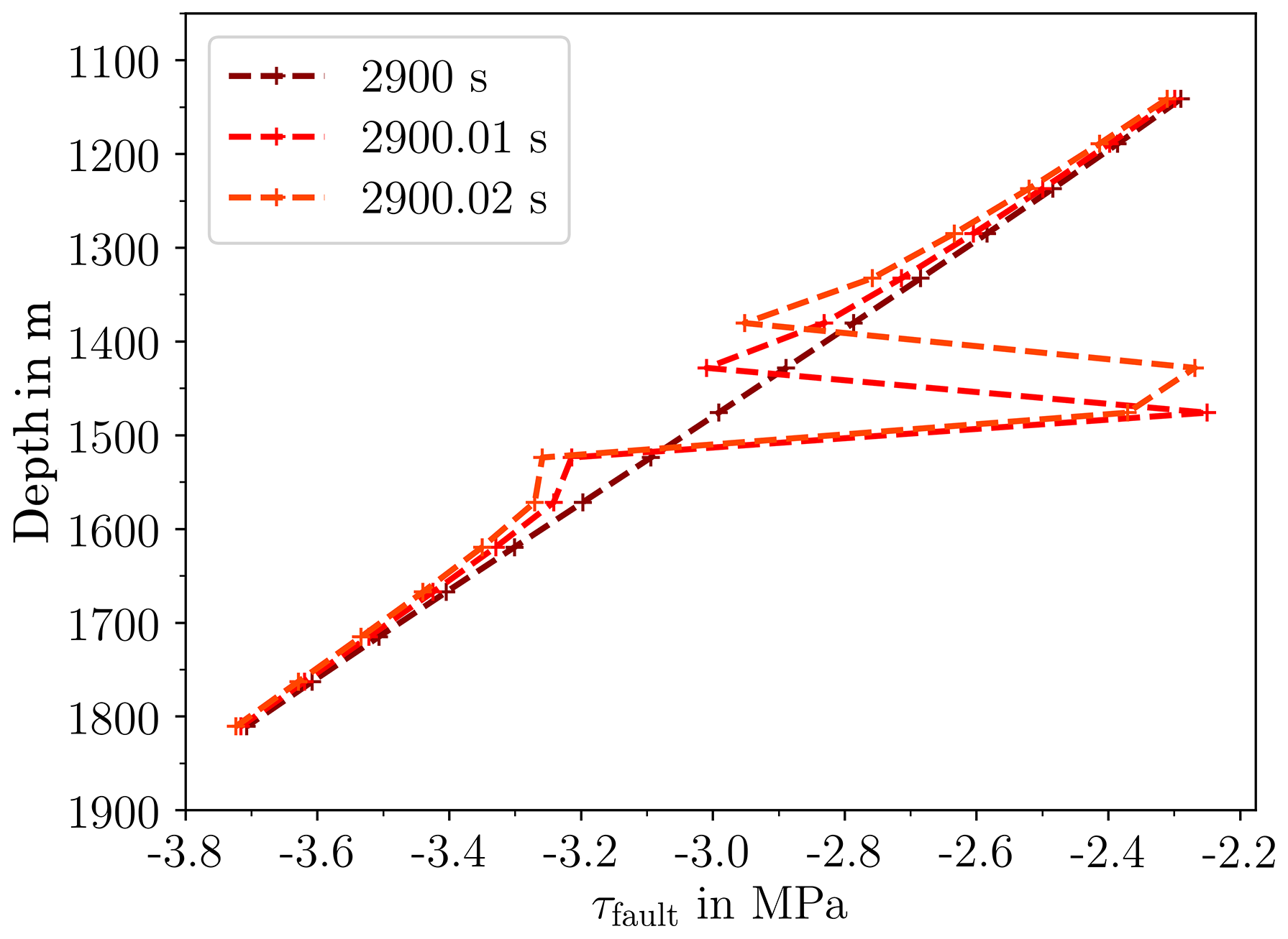
The stress drop and the following stress redistribution along the fault at time 2900 s is shown in more detail in Fig. 4. The increase of shear stress with depth is due to the boundary conditions. There is no indication for the onset of shear failure in the shear stress distribution, as this is solely caused by the reduced effective normal stress. The element at a depth of 1475 m then fails and the stress-drop is applied, leading to redistributed shear stresses, see for 2900.01 s. The neighbouring elements above and below the failed element experience an increase in shear stress. Despite of the increased shear stress, the element below resists shear failure due to a high enough normal stress resulting from the larger depth. In contrast, the element above the failed element is subjected to less normal stress and fails also. Consequently, the shear stress is reduced also for this element (at 2900.02 s). After that, no further element fails and the fault reactivation comes to a halt.
In comparison, the approach by Gómez Castro et al. (2017), at the detection of the first failing element, solves a system of equations that checks by means of stresses calculated as a response to a unit force whether failure of further elements is triggered. This is repeated until equilibrium is reached. Instead of this, we resolve time upon a failure event with very small time steps (here: 0.01 s) to achieve a quasi-simultaneous consecutive failure of several elements if necessary. Time steps re-increase immediately after a stable state is reached.
Figure 5 displays the difference in displacements for the nodes in the failed element before (only elastic deformation) and after fault reactivation (now slip!). Blue shows the nodes on the right side of the fault, red those on the left side. It can be seen that the left side moves downward, the right side upward, as can also be seen in Fig. 6. In nature, some portion of the fault slips while the remaining part, which did not fail, compensates the slip elastically. This effect can also be observed in our model. After the stress-drop is applied to the failing elements, these elements experience an increased deformation in y′-direction, which also deformes the nearest neighbours to some extent.
The obtained slip as in the right plot of Fig. 5 can be used as a measure to estimate seismic moments. Kanamori and Brodsky (2004) provide a relatively simple approach to estimate the size of an earthquake. The seismic moment M0 is estimated as M0=G A s with the shear modulus G, the mean slip s and the rupture area A. In our 2-D example, the rupture area could be estimated as a rupture length of roughly 200 m and a corresponding – e.g. circular – area, and a mean slip of 0.0026 m, as seen in Fig. 5a. Having M0, the estimated magnitude is then suggested as . With a shear modulus of 2 GPa, this would end up at a moment magnitude M=1.41 in this case.
3.2 The effect of permeability
Fault reactivation in a fluid-injection scenario is caused by the pore-pressure increase and the corresponding reduction in normal stress. Pressure response is mainly affected by permeability. Thus, we modelled two sub-scenarios with different permeability in the fault: m2 and m2.
The evolution of pressure over time is compared in Fig. 7. Failure occurs at different times, and, consequently, with different volumes injected. Lower permeabilities lead to steeper pressure gradients. Thus, at low permeabilities the pressure increase is more concentrated on the central section of the fault, while at higher permeabilities the pressure increase affects a more widespread region. This is clearly visible in the pressure margins shown (for different times in different cases!) in Fig. 7a. An important consequence thereof is that the first occurrence of failure is at different injected volumes and leads to more failed elements and larger slip in the case with higher permeability as can be seen in Fig. 8. Thus, despite the slower pressure increase and a lower maximum pressure, the expected magnitudes of the first seismic events are higher in the high-permeability case.
The hypothesis that fault reactivation can be modelled by using a characteristic stress drop between 0.1 and 1 MPa in the event of shear failure is backed up by observations for earthquakes of different magnitudes. Incorporating this into an existing fully-coupled model for flow and linear-elastic geomechanics yields consistent and plausible results and allows for a detailed analysis of the mechanisms during the reactivation of the fault. The assumption of linear-elastic behaviour is, of course, violated once an element failes. We consider this currently a small neglect in order to give a proof of concept and plan to improve this in the future.
The reduction in normal stress resulting from increased pore pressures is the key factor leading to shear failure and shear slip in the presented scenario. This is obviously linked to the shear-stress distribution prior to injection, which might, of course, be already critically charged under natural conditions.
The permeability of the formation matters for the expectable seismicity. Injection at higher permeabilities can be worse than at lower permeability. Thus, defining a maximum pressure to limit induced seismicity is no sufficient criterion. Important is also the distribution of pressure as determined by the permeability.
The implementations for this work are done in Dumux 2.12 (Fetzer et al., 2017) (https://doi.org/10.5281/zenodo.1115500) and are available for reproducing the results, see https://git.iws.uni-stuttgart.de/dumux-pub/beck2019b (Beck and Class, 2019).
MB did all the implementations, preparations of the results, and summarized them in his dissertation. HC is supervising the work and wrote this article.
The authors declare that they have no conflict of interest.
This article is part of the special issue “European Geosciences Union General Assembly 2019, EGU Division Energy, Resources & Environment (ERE)”. It is a result of the EGU General Assembly 2019, Vienna, Austria, 7–12 April 2019.
This research has been supported by the Deutsche Forschungsgemeinschaft DFG (grant nos. IRTG 1398 and SFB 1313) and the European Union (grant no. 636811 FracRisk).
This open-access publication was funded
by the University of Stuttgart.
This paper was edited by Antonio Pio Rinaldi and reviewed by Inga Berre and Victor Vilarrasa.
Abercrombie, R. and Leary, P.: Source parameters of small earthquakes recorded at 2.5 km depth, Cajon Pass, southern California: Implications for earthquake scaling, Geophys. Res. Lett., 20, 1511–1514, https://doi.org/10.1029/93GL00367, 1993. a
Aki, K.: Earthquake mechanism, Tectonophysics, 13, 423–446, https://doi.org/10.1016/0040-1951(72)90032-7, 1972. a
Beck, M.: Conceptual approaches for the analysis of coupled hydraulic and geomechanical processes, PhD thesis, Universität Stuttgart, 2019. a
Beck, M. and Class, H.: Beck2019b, source code, available at: https://git.iws.uni-stuttgart.de/dumux-pub/beck2019b, last access: 28 June 2019.
Beck, M., Seitz, G., and Class, H.: Volume-Based Modelling of Fault Reactivation in Porous Media Using a Visco-Elastic Proxy Model, Transport Porous Med., 114, 505–524, https://doi.org/10.1007/s11242-016-0663-5, 2016. a, b
Berge, R. L., Berre, I., and Keilegavlen, E.: Reactivation of Fractures in Subsurface Reservoirs – a Numerical Approach using a Static-Dynamic Friction Model, arXiv preprint arXiv:1712.06032, 2017. a
Cappa, F. and Rutqvist, J.: Modeling of coupled deformation and permeability evolution during fault reactivation induced by deep underground injection of CO2, Int. J. Greenh. Gas Con., 5, 336–346, https://doi.org/10.1016/j.ijggc.2010.08.005, 2011. a, b
De Simone, S., Carrera, J., and Vilarrasa, V.: Superposition approach to understand triggering mechanisms of post-injection induced seismicity, Geothermics, 70, 85–97, 2017. a
Ellsworth, W. L.: Injection-Induced Earthquakes, Science, 341, 1225942, https://doi.org/10.1126/science.1225942, 2013. a, b
Ferronato, M., Gambolati, G., Janna, C., and Teatini, P.: Numerical modelling of regional faults in land subsidence prediction above gas/oil reservoirs, International Journal for Numerical and Analytical Methods in Geomechanics, 32, 633–657, https://doi.org/10.1002/nag.640, 2008. a
Fetzer, T., Becker, B., Flemisch, B., Gläser, D., Heck, K., Koch, T., Schneider, M., Scholz, S., and Weishaupt, K.: DuMuX 2.12.0, 13 December 2017, https://doi.org/10.5281/zenodo.1115500, 2017. a, b
Frohlich, C., Ellsworth, W., Brown, W. A., Brunt, M., Luetgert, J., MacDonald, T., and Walter, S.: The 17 May 2012 M4.8 earthquake near Timpson, East Texas: An event possibly triggered by fluid injection, J. Geophys. Res. Sol.-Ea., 119, 581–593, https://doi.org/10.1002/2013JB010755, 2014. a
Goertz-Allmann, B., Goertz, A., and Wiemer, S.: Stress drop variations of induced earthquakes at the Basel geothermal site, Geophys. Res. Lett., 38, L09308, https://doi.org/10.1029/2011GL047498, 2011. a
Gómez Castro, B. M., De Simone, S., and Carrera, J.: A New Method to simulate Shear and Tensile Failure due to Hydraulic Fracturing Operations, in: EGU General Assembly Conference Abstracts, vol. 19 of EGU General Assembly Conference Abstracts, p. 8657, 2017. a, b
Jha, B. and Juanes, R.: Coupled multiphase flow and poromechanics: A computational model of pore pressure effects on fault slip and earthquake triggering, Water Resour. Res., 50, 3776–3808, 2014. a, b
Kanamori, H. and Anderson, D. L.: Theoretical basis of some empirical relations in seismology, B. Seismol. Soc. Am., 65, 1073–1095, 1975. a
Kanamori, H. and Brodsky, E. E.: The physics of earthquakes, Rep. Prog. Phys., 67, 1429, https://doi.org/10.1088/0034-4885/67/8/R03, 2004. a
Keranen, K. M., Savage, H. M., Abers, G. A., and Cochran, E. S.: Potentially induced earthquakes in Oklahoma, USA: Links between wastewater injection and the 2011 Mw 5.7 earthquake sequence, Geology, 41, 699, https://doi.org/10.1130/G34045.1, 2013. a
Lee, K.-K., Ellsworth, W., Giardini, D., Townend, J., Ge, S., Shimamoto, T., Yeo, I.-W., Kang, T.-S., Rhie, J., Sheen, D.-H., Chang, C., Woo, J.-U., and Langenbruch, C.: Injection-Induced Earthquakes, Science, 364, 730–732, https://doi.org/10.1126/science.aax1878, 2019. a
Rutqvist, J., Rinaldi, A. P., Cappa, F., and Moridis, G. J.: Modeling of fault reactivation and induced seismicity during hydraulic fracturing of shale-gas reservoirs, J. Petrol. Sci. Eng., 107, 31–44, 2013. a, b, c
Thatcher, W. and Hanks, T. C.: Source parameters of southern California earthquakes, J. Geophys. Res., 78, 8547–8576, 1973. a
Ucar, E., Berre, I., and Keilegavlen, E.: Three-dimensional numerical modeling of shear stimulation of fractured reservoirs, J. Geophys. Res. Sol.-Ea., 123, 3891–3908, 2018. a