 | 11 Jul 2019
Filling the gap between plot and landscape scale – eight years of soil erosion monitoring in 14 adjacent watersheds under soil conservation at Scheyern, Southern Germany
Florian Wilken
Watershed studies are essential for erosion research because they embed real agricultural practices, heterogeneity along the flow path, and realistic field sizes and layouts. An extensive literature review covering publications from 1970 to 2018 identified a prominent lack of studies, which (i) observed watersheds that are small enough to address runoff and soil delivery of individual land uses, (ii) were considerably smaller than erosive rain cells (<400 ha), (iii) accounted for the episodic nature of erosive rainfall and soil conditions by sufficiently long monitoring time series, (iv) accounted for the topographic, pedological, agricultural and meteorological variability by measuring at high spatial and temporal resolution, (v) combined many watersheds to allow comparisons, and (vi) were made available. Here we provide such a dataset comprising 8 years of comprehensive soil erosion monitoring (e.g. agricultural management, rainfall, runoff, sediment delivery). The dataset covers 14 adjoining and partly nested watersheds (sizes 0.8 to 13.7 ha), which were cultivated following integrated (four crops) and organic farming (seven crops and grassland) practices. Drivers of soil loss and runoff in all watersheds were determined with high spatial and temporal detail (e.g., soil properties are available for 156 m2 blocks, rain data with 1 min resolution, agricultural practices and soil cover with daily resolution). The long-term runoff and especially the sediment delivery data underline the dynamic and episodic nature of associated processes, controlled by highly dynamic spatial and temporal field conditions (soil properties, management, vegetation cover). On average, the largest 10 % of events lead to 85.4 % sediment delivery for all monitored watersheds. The analysis of the Scheyern dataset clearly demonstrates the distinct need for long-term monitoring in runoff and erosion studies.


Soil erosion, due to arable land use, is a major environmental threat (Montanarella et al., 2016; Pimentel, 2006) negatively affecting on-site soil properties and leading to substantial off-site damage (Pimentel and Burgess, 2013). Assessing soil erosion under natural rain can either be carried out in plot or watershed scale studies (Fig. 1). Plot studies (Fang et al., 2017; Nearing et al., 1999; Smets et al., 2009; Wischmeier, 1966) prevail in number and usually comprise a large number of plots that are simultaneously measured to account for comparability. On the other hand, watershed studies usually focus only on one or very few watersheds.
The most prominent plot set-up (the Wischmeier plots; 22.1 m long, 1.83 m wide; slope 9 %) were established while developing the still most used erosion model, the Universal Soil Loss Equation (USLE; Wischmeier and Smith, 1960). Nowadays, data of thousands of plot years of the Wischmeier plot types are available for various regions of the world. The major advantages of plot experiments are that plots are relatively easy to establish, represent a more or less homogenous area, and can be compared in paired plots (Nearing et al., 1999). The major disadvantage of plots is that they can only assess runoff generation mainly driven by surface sealing, while other processes of runoff generation like return flow are ignored. Similarly, sheet and partly rill erosion can develop on plots while (ephemeral) gullying is neglected. Furthermore, heterogeneities along the flow path, variations in slope, watershed size and soil cover (that may cause highly relevant run-on infiltration and sediment settling) are excluded in plot experiments. Furthermore, plots typically examine a narrow range of dimensions (length, width, length-to-width ratio) (Fiener et al., 2011) that differ considerably from dimensions of fields to which the results are mostly supposed to be applied (Auerswald et al., 2009, Fig. 1).
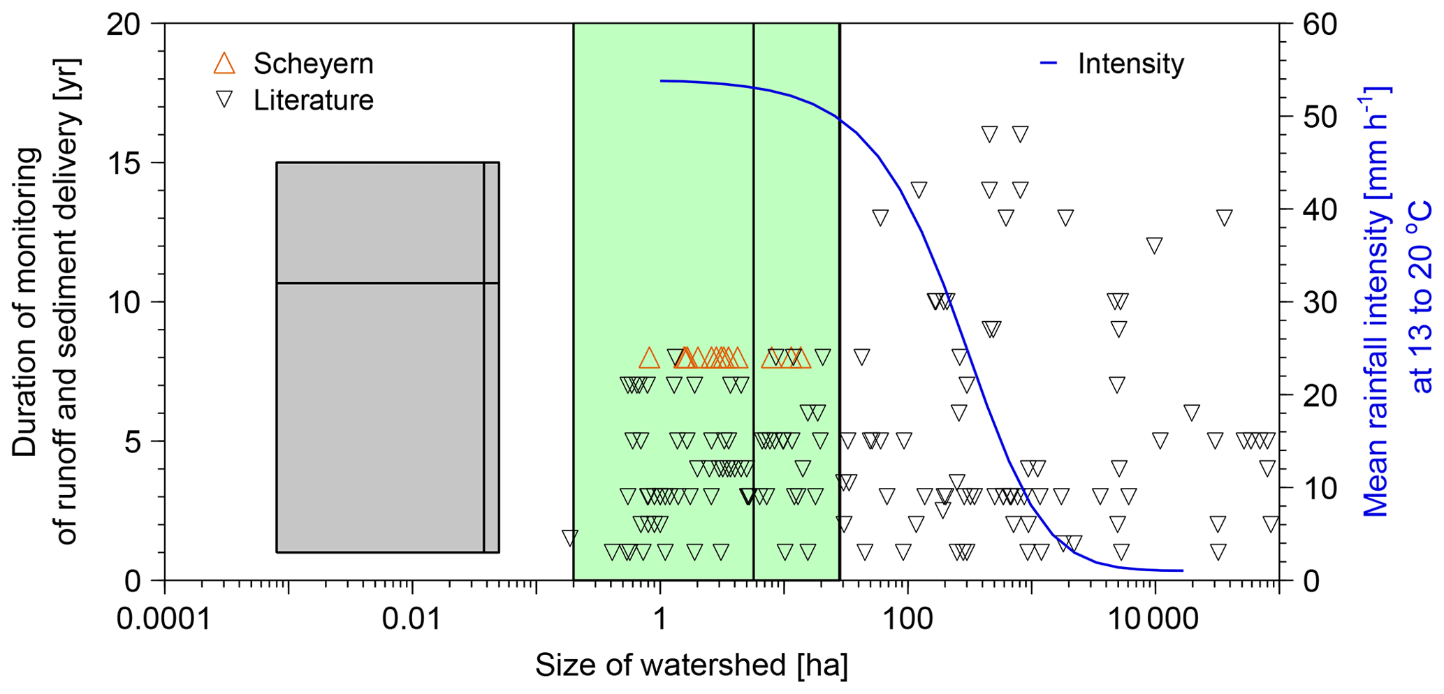
Figure 1Watershed size and duration of continuous measurements of runoff and sediment delivery for watershed studies taken from literature since 1970 (black triangles) in comparison with the Scheyern dataset (red triangles). The 99.5 %-range of field sizes in Germany is shaded in green; the vertical line denotes the average (taken from Auerswald et al., 2018). The approximate range of plot studies with natural rain is shaded in grey; the vertical and horizontal lines denote the average plot size and the average study duration (taken from Cerdan et al., 2010). Watershed studies from literature were (Anderson and Potts, 1987; Baker and Johnson, 1979; Beasley, 1979; Beasley et al., 1986; Becht and Wetzel, 1989; Bingner et al., 1989; Bowie and Bolton, 1972; Brooks et al., 2010; Casali et al., 2008; Chow et al., 1999; Deasy et al., 2011; Dendy, 1981; Dickinson and Scott, 1975; Didone et al., 2017; Diyabalanage et al., 2017; Duvert et al., 2010; Edwards et al., 1993; Evrard et al., 2008; Foster et al., 1980; Garcia-Ruiz et al., 2008; Glendell and Brazier, 2014; Grangeon et al., 2017; Hamlett et al., 1983; Hasholt, 1992; Hasholt and Styczen, 1993; Inoubli et al., 2016; Khanbilvardi and Rogowski, 1984; Kimes and Baker, 1979; McDowell et al., 1984; Mielke, 1985; Mildner and Boyce, 1979; Minella et al., 2018; Monke et al., 1979; Murphree and Mutchler, 1981; Murphree et al., 1985; Mutchler and Bowie, 1979; Nunes et al., 2016; Onstad et al., 1976; Pieri et al., 2014; Porto et al., 2009; Ramos et al., 2015; Ribolzi et al., 2017; Schilling et al., 2011; Sheridan et al., 1982; Sherriff et al., 2015; Simanton and Osborn, 1983; Simanton et al., 1980; Simanton and Renard, 1982; Sith et al., 2017; Sran et al., 2012; Starks et al., 2014; Steegen et al., 2000; Stott et al., 1986; Valentin et al., 2008; Van Oost et al., 2005; Vongvixay et al., 2018; Walling et al., 2001; Zhang et al., 2015; Zuazo et al., 2012). Note that if watershed data appear in several studies, only one study was cited here. Data to calculate the decrease in mean rainfall intensity (blue line) with increasing watershed size were taken from Lochbihler et al. (2017), who analysed the rainfall intensity for the 1000 largest rainfall events of a 9 year period (at 13 to 20 ∘C; in the Netherlands); for this figure the centre of the rainfall cell is assumed to be located in the middle of the respective watershed.
To overcome these problems, a number of watershed scale monitoring studies were carried out over the last decades (summarized in Fig. 1). They offer the advantage of sufficiently large field sizes to represent: common agricultural practices, the interaction between neighbouring sites, complex morphologies and processes like return flow from shallow ground water or subsurface flow. Thus, watershed studies offer large advantages and are an indispensable supplement of plot studies. Despite the clear advantages of watershed studies some drawbacks are inherent, which becomes clear from a comparison of such studies performed since the 1970s (Fig. 1). These studies can be distinguished into two size categories, (i) those that cover a size range that allows for a quantification of field or hillslope processes (sizes <50 ha) and (ii) those including processes in river systems (>10 km2) to represent storage and release processes of fluvial systems. However, process scale studies (i) are usually quite short and rarely exceed five years of monitoring (Fig. 1). Taking into account the large temporal and interannual variability of water erosion events (Fischer et al., 2016), this is a serious constraint. Study durations longer than five years can almost exclusively be found for watershed studies of larger scale, although short durations prevail in this size range as well (Fig. 1). An important and unavoidable trade-off associated with large watershed sizes is that internal dynamics within the river system modify the terrestrial erosion signal (Auerswald and Geist, 2018; Walling and Amos, 1999). Moreover, surface runoff and sediment delivery is sensitive to the watershed size. Particularly for the upscaling of processes from plot to landscape scale, the mechanistic understanding on field and small watershed scale is essential. However, small watershed studies are rare relative to meso-scale investigations. Furthermore, recent studies have shown that cells of high intensity rainfall only have a radius of about 2 km based on rain radar measurement (Fischer et al., 2018; Lochbihler et al., 2017). Hence, watersheds exceeding the size of 1 km2 are usually only partly covered by high-intensity rains, while larger watersheds may respond strongly to medium intensity rains of large spatial extent. Due to the increasing complexity of spatial patterns in rainfall and internal sediment redistribution and corresponding long-term storage, we restricted our review of watershed studies in Fig. 1 to watersheds <1000 km2.
A further characteristic of watershed studies in comparison to plot studies is that usually only few watersheds are compared. Numerous monitoring studies have been carried out in single watersheds (see all watershed sizes in Fig. 1 with unique study duration). Furthermore, the majority of studies do not compare more than three watersheds. This small number limits a direct comparison and usually does not allow for an analysis of the influence of spatial variability in watershed properties. Thus, it does not surprise that all watershed studies found in literature report a rather superficial description of topographic, pedologic and agronomic properties of the watersheds and of the meteorological conditions during the study period. This becomes evident when compared to plot studies that at least describe in detail plot morphology, soil properties and agricultural treatment. The lack in a detailed description of boundary conditions also impedes the combination of data from different studies, although this would greatly increase the value of such studies. Unfortunately, a combination and comparison of different watershed studies is impossible because sufficient data are usually not reported.
Here we report about the Scheyern dataset that overcomes some of the limitations in watershed studies. (i) The dataset allows for the comparison of a large number of adjacent and partly cascading watersheds (14) that are amended by many plot data under simulated rainfall. (ii) It covers a relatively long study period (8 years). (iii) The dataset is available and can be used for comparisons within this dataset, against other datasets or modelling results (for data overview see Table 1). (iv) All watershed sizes are within the range of fields and hillslopes and thus exclude interference of processes along the aquatic flow path. (v) Finally and importantly the data of soil loss and runoff during erosion events are complemented by a very detailed set of soil properties (e.g., spatial resolution of 12.5 m×12.5 m), weather data (e.g., tipping bucket rainfall is for some years available up to a spatial resolution of 11 km−2), agronomic data (all agricultural operations were recorded), soil cover data and topographic conditions. Based on this comprehensive dataset, we illustrate the importance of long-term monitoring and of internal temporal dynamics for interpreting watershed deliveries (e.g. the gradual and asynchronous vegetation cover development on individual fields within a watershed that additionally experience abrupt changes due to agricultural management and/or may receive different amounts of erosive rain due to small scale variability in rainfall depths).
2.1 Test site
The Scheyern Experimental Farm was located about 40 km north of Munich, Germany. The test site covered an area of approximately 150 ha (Fig. 2) and is part of the Tertiary hills, an important agricultural landscape in Central Europe. The Tertiary sediments are mainly sandy to gravelly, quarzitic, fluviatile materials of poor fertility. Especially hilltops are often covered by shallow clayey sediments (either calciferous or not) of former oxbow lakes in the fluviatile Tertiary landscape. Hills were developed during the Pleistocene within these horizontally deposited Tertiary sediments. These hills are steep on the warm south and west facing slopes due to erosion facilitated by the lack of permafrost. The cold east and north facing slopes had permafrost and solifluction that left gentle slopes. Furthermore the gentle east facing slopes received some loess (0 to 2 m), which made them suitable for cropland, which in turn lead to colluvial soils in toe slope positions (Sinowski and Auerswald, 1999). As a result of these formation conditions, the research area exhibits a wide range of soils, from shallow to deep, from gravelly to sandy to silty to clayey and a wide range of slope gradients. Well-sorted textures dominate in sediments at greater depths (>30 cm) while surface soils are poorly sorted and loamy textures dominate (Auerswald et al., 2001). Following the IUSS Working Group WRB (WRB, 2015), soils at the research farm are classified Haplic Luvisols, Endogleyic or Haplic or Leptic Cambisols, Gleyic or Haplic Fluvisols, Mollic Gleysols.
Table 1Structure of the Scheyern data base. The zip-files (bold) combine all data and meta-data within one topic, with an individual DOI. Each zip-file contains several csv files with data, shape files (which are zipped) for geographic information and corresponding pdf files describing the meta-data.
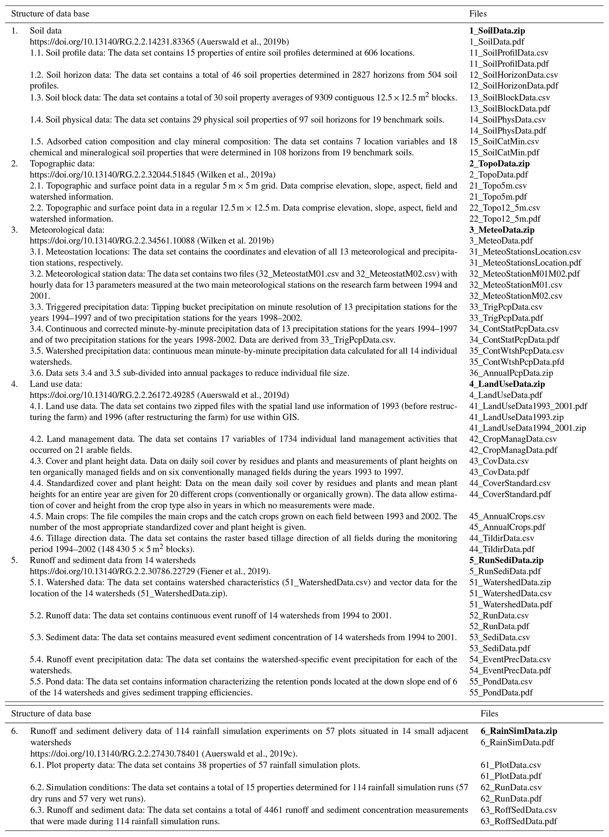

Figure 2Land use and monitored watersheds at the research farm (without area for cropping experiments). Numbers ≤6 indicate integrated management, numbers ≥7 indicate organic management.
The elevation ranged from 448 to 497 m above sea level with a mean slope of 10.1 % (±6.1 %). Slopes facing south and east were gentle (approx. 10 %) while in contrast the slopes facing north and west are partly much steeper (up to 30 %). An intense tachymetric survey was conducted to determine slope angles and watershed boundaries, whereas precise elevation was recorded at approximately 4500 positions (30 measurements per ha); for details see Warren et al. (2004). Moreover, a 5 m×5 m LiDAR digital elevation model (DEM) is available. The watershed borders were determined from tachymetric survey and in-situ runoff tracking during long-lasting runoff events (snowmelt). This was necessary as the LiDAR DEM did not properly resolve watershed borders due to small scale structures like tillage induced roughness and grassed ditches along field borders.
The climate was temperate humid with a mean annual air temperature of 8.4 ∘C during the monitoring phase from 1994 to 2001. The average precipitation was 804 mm yr−1 (1994–2001) with the highest precipitation occurring from May to July (average maximum 116 mm per month in July) and the lowest occurring in the winter months (average minimum 33 mm per month in January). The mean annual erosivity was 97 (Auerswald et al., 2019a).
At the research farm, two types of farming systems (conventional and organic farming) were established after harvest in 1992. The border between both farming systems followed the main watershed boundary in order to have only one system within a certain watershed. One system followed the principles of conventional integrated farming (total size: 46 ha) (not to be confused with the European agriculture organic standard of integrated farming) and the other followed certified organic farming according to the rules of the German Association for Ecological farming (AGOL; total size: 68 ha). In general, the organic farming was located in areas with higher soil variability, partly situated at steeper slopes (mainly grazed) and on less productive soils compared to the fields of integrated farming. The higher soil variability and the steeper slopes required smaller field sizes. Methodologically this was advantageous, because it allowed for the cultivation of two fields with the same crop every year despite the more complex crop rotation. Thus, in both farm types each crop was replicated in each year. The remaining area of the farm was used for cropping studies, where treatments were applied that would have been in conflict with the initially defined and continuously applied land use principles of the two farming systems.
In general, integrated farming and organic farming allow a wide range of management options. The management of both farming systems at the research farm aimed to improve in parallel the economic returns and soil protection (i.e., minimizing erosion and soil compaction), water protection (i.e., minimizing leaching of agrochemicals), and of biodiversity enhancement (Auerswald et al., 2000). This multiple-goal approach required a set of sophisticated and rather unusual management options like the use of ultra-wide tires on light tractors or avoiding temporal gaps in soil cover by consequent application of cover crops, catch crops and residues management. Hence, the management in both systems differed considerably from what can be found on typical farms that also apply integrated or organic farming.
The 4-year crop rotation in the integrated farming system was potato (Solanum tuberosum L.), winter wheat (Triticum aestivum L.), maize (Zea mays L.), and winter wheat. The organic farming system had a 7-year crop rotation starting with a grass-clover mixture (typically containing perennial ryegrass Lolium perenne L., Italian rye-grass Lolium multiflorum Lam., meadow fescue Festuca pratensis Huds., red clover Trifolium pratense L., and white clover Trifolium repens L.) and followed by potato, winter wheat, winter rye (Secale cereale L.), white lupine (Lupinus albus L.), and sunflowers (Helianthus annuus L.) (Auerswald et al., 2000). To meet the rules of nutrient use of the AGOL, the organic farm ran a herd of 30 suckler cows with a bull. The cattle were grazing the pastures during summer (for details see Auerswald et al., 2010; Schnyder et al., 2010), whereas manure from the winter stall period was used for fertilizing the organic fields. In the integrated system, maize was produced that was externally used to feed 49 steers. The slurry from this herd was applied as manure at the integrated farming system.
In order to reduce surface runoff and sediment-bound matter fluxes, land use and soil management were adapted (see below) and a number of near-field buffer features were installed. The latter mainly comprised small retention ponds with sub-surface outflows at the downslope end of the watersheds W01, W02, W05, W06 and W14 (Fig. 2). The retention ponds were designed to retain water for a maximum of three days with extreme events (for details see Fiener et al., 2005). A grassed waterway to prevent ephemeral gullying and reducing surface runoff was established in 1993 in the watersheds W05 and W06 (for details see Fiener and Auerswald, 2003).
The main cropping principle in both farming systems was to keep the soil cover high as long as possible, preferably by growing plants or plant residues where this was not possible. This intended to lower nitrate leaching and erosion but also to increase the input of organic matter into the soil food chain. To this end, cover crops were sown and mulch tillage (Kainz, 1989) was applied in the integrated system while catch crops were used in the organic system. Also unconventional methods were applied, e.g. sowing mustard (Sinapsis alba L.) into potato fields, when the potato leaf cover at the end of the growing season decreased due to Phythophtora infestans infection (Kainz et al., 1997). To prevent soil compaction and allow reduced tillage, it was necessary using the lightest machinery for a given task and using ultra-wide tires on all farming machinery. Mouldboard ploughs were used that allowed to run with both wheel tracks on the unploughed land, while with the usual mouldboard plough one wheel runs on the subsoil of the furrow and compacts the subsoil; non-inverting shallow-depth tillage and stabilization of the soil structure by increasing biological activity further assisted this concept (Auerswald et al., 2000).
2.2 Data
2.2.1 Soil management and soil cover
Any soil and crop management performed at one of the 23 arable fields was documented by the farm manager. The available data comprise e.g. sowing date, sowing density, crop type and sowing machinery. Any application of fertilizer and agro-chemicals was documented including date, machinery used, type of fertilizer and/or agro-chemical, amounts etc.
During the 8 year monitoring period, plant and residue cover was measured for 3 1/2 years (January 1993 to April 1997) in all fields. During the vegetation period, measurements were carried out bi-weekly; during autumn to spring cover was measured monthly and additionally before and after each soil management operation. Measurements were repeated at a minimum of three geodetically defined locations within each field. Residue cover and cover of plants near the surface were measured manually using a meter stick. Plant height was also determined with a meter stick. Plant cover of higher plants were derived from photographs taken around noon from a height up to 4 m (in the case of full-grown maize) using image analysis (Kaemmerer, 2000).
2.2.2 Soil
A combination of geostatistics and pedotransfer-functions were used to determine the spatial distribution of important soil properties in three dimensions and at high resolution (Scheinost et al., 1997). Therefore, soil sampling in a rectangular 50 m×50 m grid (471 grid nodes) using a machine-auger down to a depth of 1.2 m with a soil core diameter of 0.1 m was carried out. In total 2448 soil horizons were sampled and analysed for texture, plant available P and K according to Schüller (1969), pH in 0.01 M CaCl, total and carbonate C by dry combustion, and total N. Soil texture was determined for 3 stone fractions and 15 fine earth fractions (Auerswald and Schimmack, 2000). Additionally 19 benchmark soils between the grid nodes were sampled and analysed in more detail. In areas of steep gradients between grid node soils, additional hand augering was applied for soil categorization using field methods (for more details regarding soil sampling and analysis see Auerswald et al., 2001; Scheinost et al., 1997; Sinowski et al., 1997).
All soil data were combined in an extensive geostatistical analysis to interpolate soil properties, e.g. C content and texture, for 12.5 m×12.5 m grid blocks. For details of the procedure see Scheinost et al. (1997). The geostatistical interpolation scheme was also applied to derive a high resolution K factor map, which is used in this study to illustrate the richness of the data set and also to underline the importance to account for spatial variability within watersheds to understand differences in hydrological properties. The K factor was determined at 544 locations (471 grid nodes and 73 points in-between the grid nodes) according to the K factor nomograph (Wischmeier et al., 1971). Bulk soil fractions (in %) of silt (fSi), very fine sand (fvfSa), clay (fCl) and organic matter (fOM) in the fine earth fraction and the fraction of rock fragments (frf) were measured; aggregate size class (a) was obtained by visual classification; permeability class (p) was estimated from saturated conductivity calculated by using a pedotransfer function that had been developed from measured saturated conductivities of 737 soil cores taken from various soils and horizons at the research farm. The range of soils exceeded the validity range of the K factor equation given by Wischmeier and Smith (1978). In order to avoid manual reading of the K factor nomograph for 544 soils, we used the K factor equation by Auerswald et al. (2014) that includes all peculiarities of the nomograph, which are not included in the simpler equation by Wischmeier and Smith (1978). It is a combination of 4 equations; note that there were typing errors in the original publication by Auerswald et al. (2014); we used the correct equations:
These equations use the unit [] for K and the interim values K1 to K3. The unit can be converted to the unit [], commonly used in the USA, by dividing by 10. Subsequently, the K factor was geostatistically interpolated for 12.5 m×12.5 m blocks using the gstat package (version 1.1-6; Gräler et al., 2016; version 3.5.0; R-Core-Team, 2018).
2.2.3 Weather
Hourly climate variables were measured at two meteorological stations located at the research farm from 1 April 1994 to the 31 December 2001 (for location see Fig. 2). Data from a nearby meteorological station of the German Weather Service Voglried (approx. 3 km north of the research farm) were included to complete the 8 year monitoring data set for the time span 1 January to 31 March 1994 and to fill gaps in the data from the research farm for the time span 13 August 1999 to 7 July 2000. The meteorological stations provided the following standard variables: air temperature and relative humidity measured at 0.5 and 2.0 m above ground; global radiation, wind speed and wind direction at 2.0 m above ground; soil temperature and moisture under grass at depths of 0.05 and 0.5 m; precipitation in 1.0 m above ground. Precipitation at both stations was recorded with tipping buckets (resolution 0.2 mm; collecting area 0.04 m2; measuring height 1.0 m) from the 1 April 1994 onwards. Precipitation was additionally measured at 11 stations (resolution 0.1–0.2 mm; collecting area 0.02 m2; measuring height 1.0 m), which were located more or less equally distributed over the research farm, to capture the spatial variability of (erosive) rainfall events between April 1994 and March 1998. Eight of the overall 13 rain gauges at the research site were heated, to measure precipitation continuously also in case of snowfall during the winter months. The tipping-bucket rainfall data of all stations were recorded in minute temporal resolution (more details regarding this dataset and the spatial distribution of rainfall is given in Fiener and Auerswald, 2009).
Table 2Watershed land use and mean topsoil properties based on a 50×50 m inventory in 1992 geostatistically interpolated to a raster of 12.5×12.5 m (Scheinost et al., 1997).

a proportion of fine earth <2 mm; clay <2 µm, silt 2 to 63 µm; b proportion of total soil including stones
2.2.4 Surface runoff and sediment delivery
Surface runoff and sediment delivery was continuously monitored for all events at the outlet of 14 watersheds (Fig. 2; Table 2) from 1994 to 2001. All watershed outlets collected surface runoff by small dams that transmitted runoff via an underground-tile outlet (diameter of pipes 15.6 and 29 cm) to the measuring device. In case of W01, W02, W05, W06 and W014 the peak surface runoff rates were dampened by 4 cm effective opening widths of the underground-tile outlets, thus the small dams acted as small retention ponds (volumes: W01=420 m3, W02=490 m3, W05=340 m3, W06=220 m3, W14=43 m3). For this study, only sediment delivery data at the outlet of the watersheds are analysed; it is important to note, especially in case of comparing watersheds with and without ponds, that the ponding resulted in substantial sediment trapping, which was determined after the first monitoring year. The average trapping efficiency of the main ponds (W01/02/05/06) was 56 % (Fiener et al., 2005).
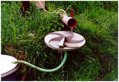
Figure 3Coshocton-type wheel surface runoff sampling device and collecting tank used to monitor surface runoff and sediment delivery at all watershed outlets.
From the underground-tile outlet pipes, the surface runoff was channelled to Coshocton-type wheel surface runoff samplers. The setup is similar to that used by Carter and Parsons (1967), collecting an aliquot of 0.5 % from the outlet surface runoff (Fig. 3). The aliquot precision of the Coshocton wheel setup was tested in a laboratory flume. The measured aliquot showed reliable precision in the range of ±10 % of the intended aliquot (for more details regarding the precision of the measuring set-up see Fiener and Auerswald, 2003).
The aliquot volumes were collected in 1.0 to 3.5 m3 tanks and measured after or during (large) surface runoff events. During water and sediment sampling, the tank content was vigorously mixed using a submersible pump to homogenize sediment concertation before water samples were taken. Subsequently, the water samples were dried at 105 ∘C to determine sediment concentrations. In 1995 some of the collecting tanks (at W01, W02, and W06) were replaced by tipping buckets (volume = approximately 85 mL) at the outlets of the aliquot wheels. The tipping buckets were connected to Model 3700 portable samplers (Isco, Lincoln, NE) that counted the number of tips and automatically collected a surface runoff sample after a defined runoff volume (Fiener and Auerswald, 2003). This modification (used for those watersheds that produced most surface runoff) resulted in more data per event, which provides more information on intra event dynamics. We limited the data set used in this study to total event runoff volumes and sediment delivery as inter event data is not available for all watersheds and measurements. However, the corresponding data publication (Fiener et al., 2019) covers the sub-event information.
An individual event number and corresponding time span was assigned if at least one watershed recorded surface runoff. If more than one watershed produced runoff, the time span between the first recorded runoff in one of the watersheds and the last recorded runoff in one of the watersheds was associated to the event number. This simple definition can lead to prolonged runoff events that consist of a series of precipitation events as runoff events of different watersheds may overlap. Especially during winter events, a clear definition of events was partly difficult as some watersheds produced prolonged surface runoff resulting from return flow. Within the dataset, detected errors are flagged, e.g. in case of large events, the runoff tanks needed to be emptied during the events that led to a slight underestimation of runoff and sediment delivery volumes.
2.2.5 Rainfall simulation data
The natural rainfall data were complemented by rainfall simulation data that were obtained before the monitoring period under natural rain started. At 57 plots within the studied watersheds, a simulation was performed on dry soils (dry runs) lasting 60 min at a mean intensity of 64 mm h−1 using a Veejet 80100 rainfall simulator (the so-called Kainz-and-Eicher simulator; Kainz et al., 1992). The rainfall simulator applies rainfall kinetic energy of 20 . Following the standard protocol of Auerswald et al. (1992), at all 57 plots an additional very wet run under pre-sealed soil conditions was applied. This very wet run started 30 min after the end of the initial dry run and applied 30 min rainfall. The rainfall simulations were carried out immediately after harvest. For plot preparation, above-ground crop residues were carefully removed, the soil was tilled, and seedbed was prepared using a rotary harrow. The plot installation followed the standard of Auerswald et al. (1992) with the exception that plot width covered half the working width (1.5 m) of the rotary harrow (wheel track included). With regards to similar aging conditions of aggregate stability for all plots (Auerswald, 1993), seedbed preparation was carried out less than three hours before the dry runs started. Soil moisture was determined before the start of the dry run. Soil cover by stones and residues was determined before the dry run and after the very wet run. Surface roughness, following Morgan et al. (1998), was determined before the dry run started. Soil properties were measured for each individual plot. Slope steepness was determined with a water level on each plot (Warren et al., 2004). Time to ponding was determined according to the first occurrence of a soil surface water film that did not disappear between two subsequent sprays of the nozzles. Time to runoff was defined as the first continuous runoff leaving the gutter at the lower end of the plot. The plot coordinates denote the centrum of the plots and were geodetically determined (accuracy <2 cm). The runoff data have been already analysed by Fiener et al. (2013).
2.2.6 Statistics and data availability
Apart from the geostatistical analysis described above, the statistical analysis was performed with CoStat 6.451 (CoHort Software, US). Mean values are often given with standard deviation (SD) (mean ± SD). In some cases other basic statistical measures of variability were calculated as well (e.g., intervals of confidence; range, minimum and maximum, skewness) that all followed standard methods (Sachs, 1984). Although the data were in most cases highly skewed (skewness between 4 and 9) and should be transformed prior to statistical analysis, we analysed the untransformed data because they are easier to report and we only intend to give a general description of the dataset without hypothesis testing (the untransformed data carry the usual units; they have symmetric confidence bands; they do not require different transformations for different watersheds). However, this makes comparison troublesome; a transformation is hardly possible when all events are included, even if they did not produce runoff and sediment delivery in a specific watershed, because a log transformation is then not possible anymore and often bimodal distributions resulted.
A total of 287 events produced runoff in at least one of the watersheds. In most cases, not all watersheds produced runoff during an event and hence the number of events per watershed was lower and differed considerably between watersheds (69 to 275 in total or 9 to 36 events per year, Table 3). The mean runoff per event differed between 0.12 and 2.49 mm (mean 1.17 mm). The surface runoff ratio (cumulative surface runoff ∕ cumulative precipitation) during the 8 years monitoring in the different watersheds ranged between 0.2 % and 7.8 % (mean 3.0 %±2.3 %). In comparison, those watersheds of only few runoff events did not necessarily produce the lowest runoff per event. This indicated substantial variation among the events within a watershed. The coefficient of variation for event runoff varied between 200 % and 700 % (mean 365 %) for the individual watersheds. For a 1-year measuring period, the mean event runoff could only be predicted with a 95 % interval of confidence of ±183 % around the mean. In other words, it is hardly possible to derive a reasonable mean of erosion from a 1-year study period. This is also true for a 3-year study period, which is a commonly found monitoring period in soil erosion studies. The mean 95 % interval of confidence for a 3-year period would be ±99 % (ranging up to ±183 % for individual watersheds). The uncertainty was still large at the full 8-year study period with a mean 95 % interval of confidence of ±60 % (ranging up to ±111 % for individual watersheds). Statistical uncertainty was even higher for sediment delivery. In this case, the mean coefficient of variation was 477 % (compared to 365 % for runoff), which means that also the confidence bands around the mean would be about 1.5 times higher than those reported for runoff. Remarkably, the width of the confidence band correlated only weakly with site or land use conditions, e.g. the variation in watersheds dominated by grass was not smaller than the variation in watersheds dominated by arable use (variation expressed in percent of mean). Hence, in ecosystems of episodically occurring erosive rainfall, short monitoring periods may enhance the mechanistic understanding of soil erosion processes but do not support predictions on long-term soil erosion rates.
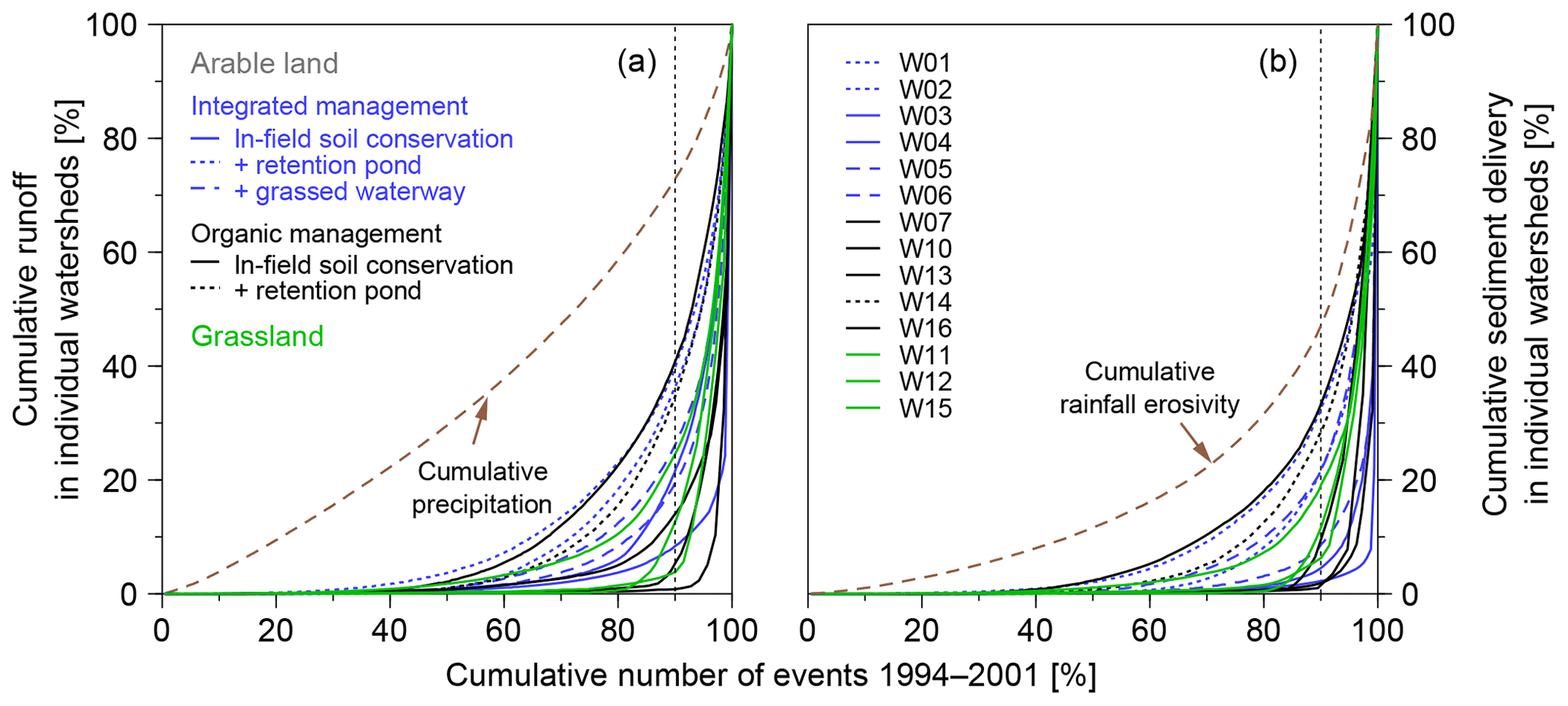
Figure 4Cumulative event surface runoff (a) and sediment delivery (b) for all watersheds versus the number of observed events in each individual watershed between 1994 and 2001 (except for watershed W11: 1998–2001; and watershed W04 due to an error in most extreme event). All cumulative events are sorted in ascending order. Cumulative precipitation and erosivity is calculated for all erosive events; erosivity was determined following Schwertmann et al. (1987).
Skewness was considerably higher for sediment delivery compared to runoff while highest skewness was found between the different watersheds (range 4 to 13). This large skewness resulted from the fact that among all watersheds at least 50 % of surface runoff did occur in only 10 % of the events (mean 75.8 %±14.7 %; Fig. 4a). At least 67 % of all sediment was delivered by the largest 10 % of events while the mean of all watersheds is substantially higher (mean 85.4 %±11.5 %; Fig. 4b). Large events were also much more important for sediment delivery than for rainfall erosivity (largest 10 % of erosive rainfall events represent 53 % of cumulative erosivity, Fig. 4b). This is because the variability of sediment delivery depends on the variability of rain events but also on the variability of soil cover. Extreme soil erosion was limited to heavy rainfall events that hit seldom and short periods of low soil cover. The general behaviour that especially soil erosion and sediment delivery is governed by extreme events was also found in plot experiments (Nearing et al., 1999), and is also demonstrated in the analysis of single extreme events on plot (Martinez-Casasnovas et al., 2002) and watershed scale (Coppus and Imeson, 2002).
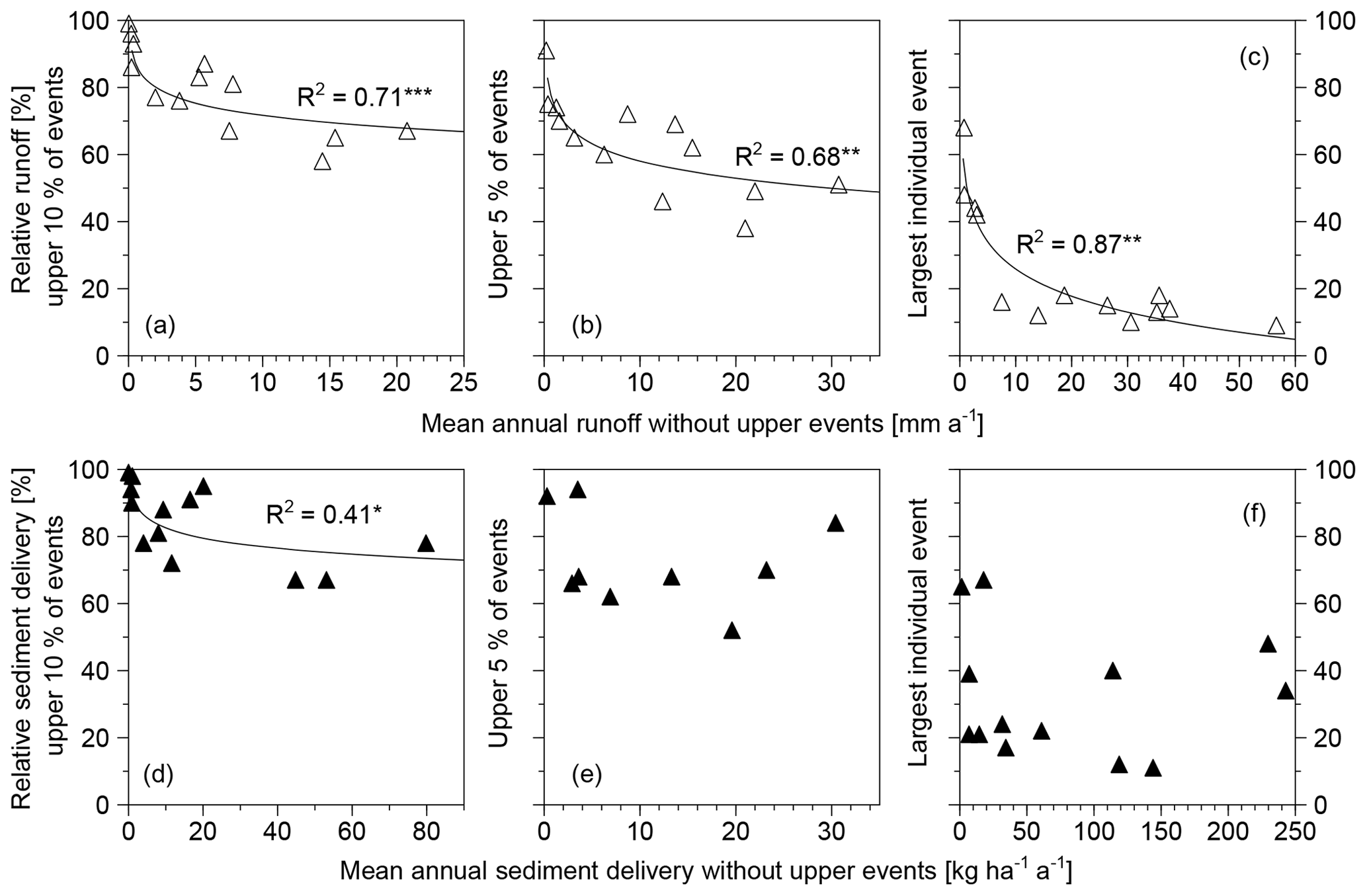
Figure 5Relation between the upper 10 % (a, d), 5 % (b, e) and the largest (c, f) surface runoff and sediment delivery events and mean surface runoff and sediment delivery in each watershed without the upper 10 %, 5 % or the largest events. Except for watershed W04 due to a measurement failure for the most extreme event. Insignificant regressions were omitted.
In the Scheyern dataset, the proportion of large surface runoff events in total runoff correlates negatively with the total runoff without these large events. This indicates that watersheds with small surface runoff sums were more dominated by extreme events (Fig. 5a–c). Hence, longer monitoring periods are required for watersheds of low runoff potential, either because of site conditions (no severe rains; permeable soils) or because of land-use conditions. A similar behaviour was not evident in case of sediment delivery. Neither the largest 5 % of all sediment delivery events nor the largest individual events showed a significant correlation to the cumulative sediment delivery of a watershed (Fig. 5d–f). This is because low sediment deliveries were always associated with a continuously large soil cover. Hence, there was less variation in such watersheds than in watersheds that produce high soil loss due to periods of little soil cover.
Especially for sediment delivery, the majority of cumulative 8-year sediment delivery was caused by large events. To assess the drivers of extreme events, we will focus in the following on the importance of monitoring the internal dynamics of watersheds. From the fact that the total number of rainfall events was considerably larger than the number of runoff events already follows that in some cases a watershed must have produced runoff while others did not. Such events can only be understood if land use, spatial rainfall distribution and site conditions are known in detail. This dataset study comprises such data in unprecedented detail, which is illustrated by event #229 in watershed W03 that produced the largest sediment delivery per hectare for all watersheds during the entire monitoring period. The event rainfall erosivity was only 9.7 N h−1, which is one tenth of the mean annual erosivity. This event did not result in substantial erosion in the other watersheds. This extreme event was able to take place because the field in W03 was at seedbed conditions for winter wheat after potato had been harvested four weeks earlier. Therefore, the field had no soil cover at all (see arrow Fig. 6) and the soil structure was substantially damaged by potato harvest. Furthermore, a smaller event one week before the extreme event (#228) had already produced a rill network, which increased the sediment connectivity during the largest event. Both events together comprised 61.4 % of all sediment delivery measured during the 8 years in watershed W03. Watershed W03 was under integrated arable management, which in general, produced the largest events, while arable land and grassland under organic management showed substantially lower event-based sediment delivery (Table 4). Under organic management, all extremes (except for W15) occurred in late winter to early spring and were associated with snowmelt and/or prolonged rainfall with minor event rainfall erosivity (Table 4). In contrast, extremes (except for W06 which produced anyway very small sediment delivery rates (Tables 3, 4)) under integrated farming were associated with large erosivities and times of low soil cover similar to event #229 in W03.
Table 3Characteristics of measured surface runoff and sediment delivery events (W01 … W07, W10, W12 … W16: 1994–2001; W11: 1998–2001) in the different watersheds; C.V. is coefficient of variation. “Sum” is the total of eight years while all other columns are event based. In total 287 events were recorded that produced runoff in at least one of the watersheds.
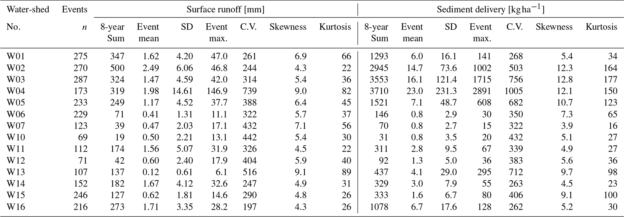
Table 4Conditions during the largest sediment delivery events measured in each watershed between 1994 and 2001.
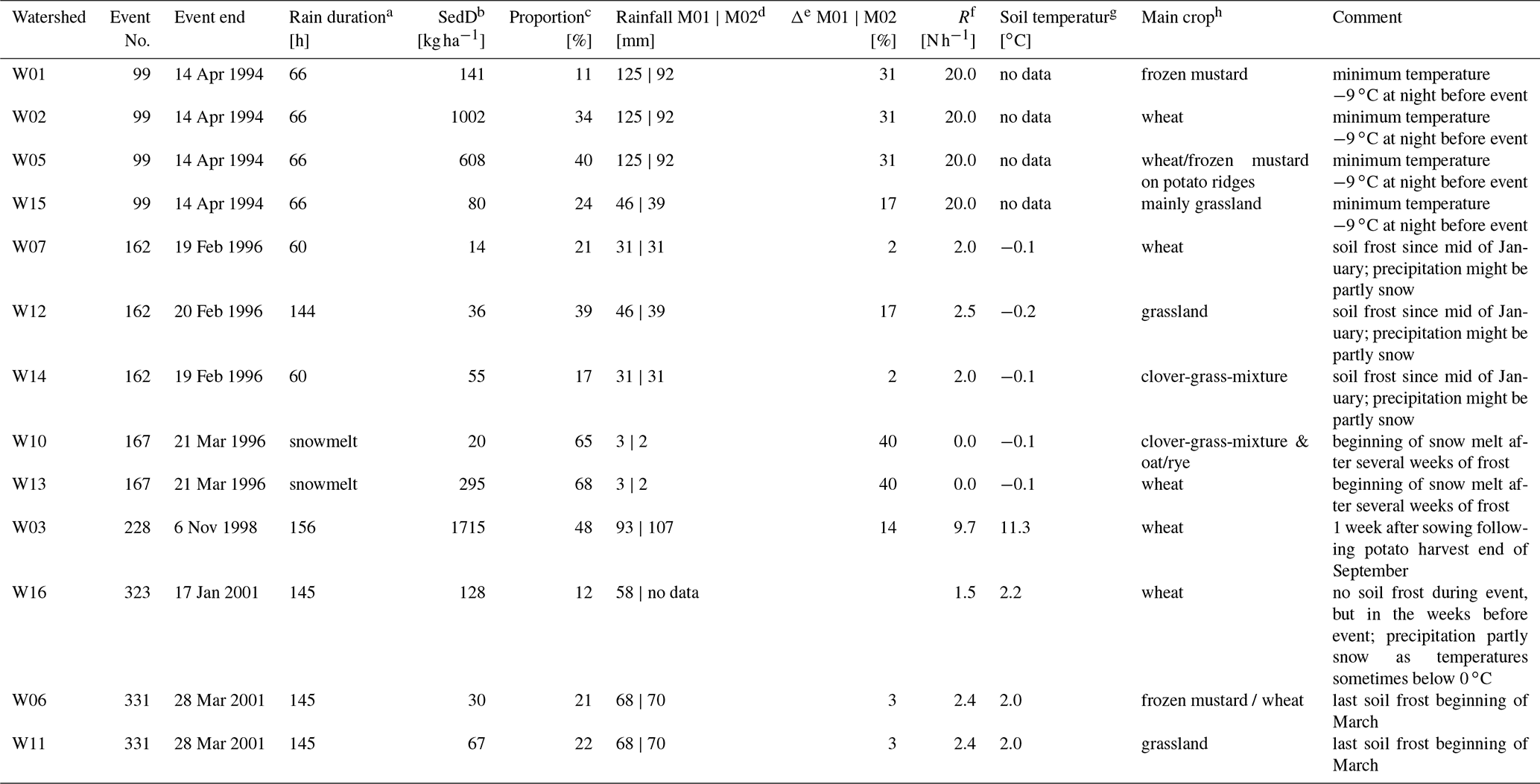
a Start of rainfall till last rainfall during surface runoff
b Sediment delivery
c Contribution of event to 8-year sediment delivery
d Event rainfall at meteorological stations M01 and M02
e Relative difference in event rainfall between stations M01 and M02
calculated as
f R factor (the unit N h−1 can be converted to MJ
by multiplication with 10)
g At the beginning of the event
h In case of two fields in the watershed the two crops are separated by a
slash; “frozen mustard” means a frozen-down catch crop; wheat and rye were
sown in fall while oat was sown in spring
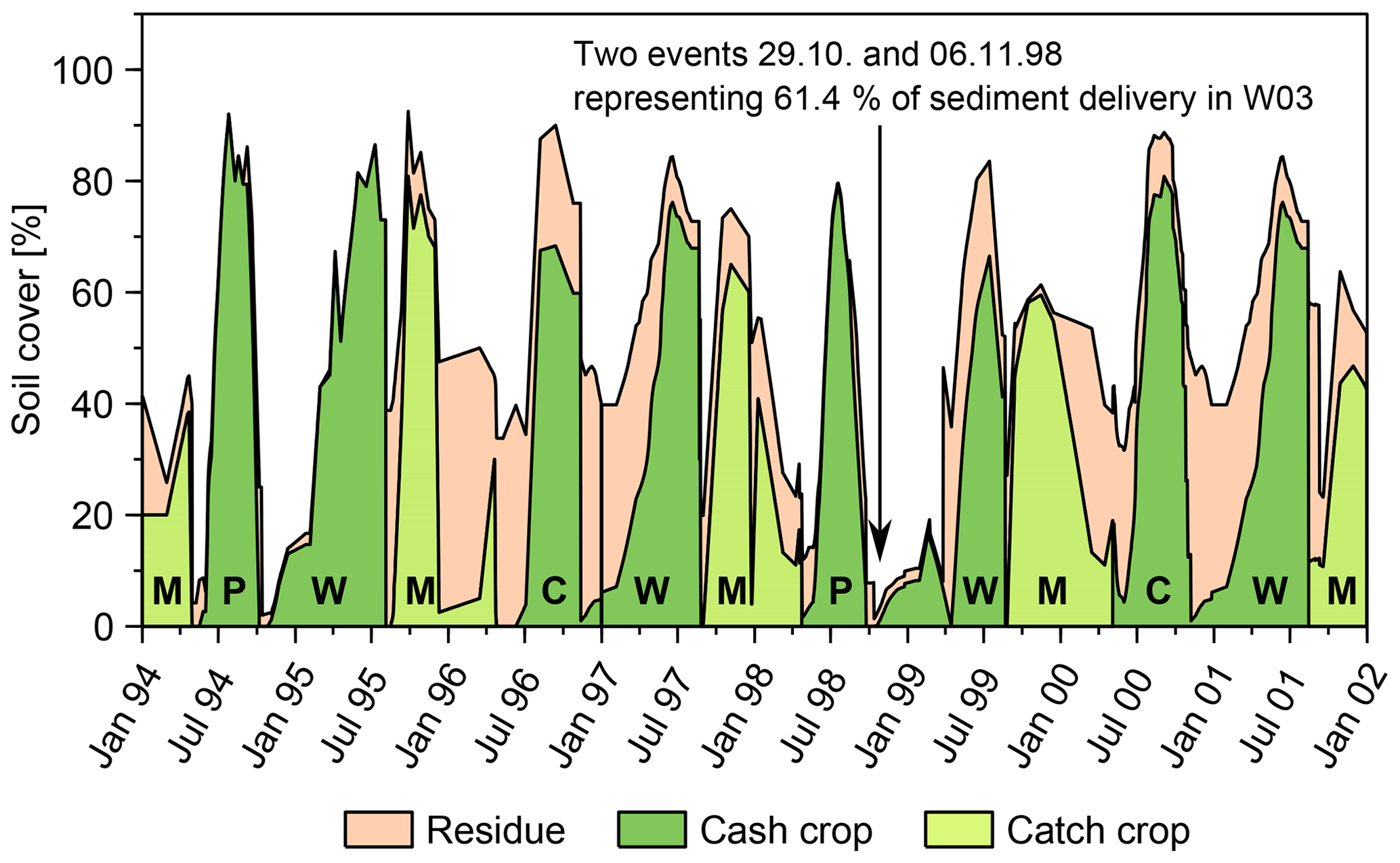
Figure 6Averaged soil cover derived from measurements within the field drained by watersheds W03 and W04; between 1994 and 1996 the cover was measured; from 1997 to 2001 the soil cover was derived from the average cover measurements (1994–1996), taking into account the crop and the year-specific times of field operations within the test field occurring from 1997 to 2001 (W: wheat, C: maize, P: potato, M: mustard used as catch crop) (modified after Fiener et al., 2008). The arrow indicates the timing of the combined largest two soil delivery events in this watershed.
Without such detailed watershed data, it is hardly possible to understand the processes driving such a series of large events. A lack of such detailed data becomes especially critical if runoff and sediment delivery data are used for model development and testing. Large events play an essential role in model development, calibration, and testing to ensure a robust prediction of extremes that are mostly of highest relevance.
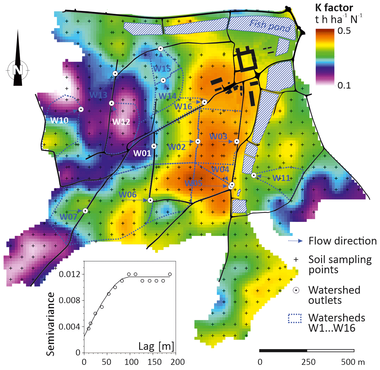
Figure 7K factor map of the research farm; K factor was determined according to Wischmeier et al. (1971) at the sampling locations from measured soil properties and then geostatistically interpolated for 12.5 m×12.5 m blocks. The krige standard deviation was about 0.02 . The small panel displays the experimental semivariogram calculated from 544 sampling locations and a spherical semivariogram model.
Equally important as the temporal dynamics of farming activities that affect soil cover and other properties are detailed data regarding spatial and spatio-temporal variability of natural drivers. Within short distances almost the entire range of soil erodibilities can be found in the study area (Fig. 7). The K factor at the grid nodes ranged from 0.03 to 0.65 , while it ranged from 0.09 to 0.47 for the 12.5 m×12.5 m blocks (Fig. 7) derived from the grid nodes. Only 3.5 % of all 20 000 soils covering Germany, that were analysed by Auerswald et al. (2014), had a K factor outside this range that can already be found within the 150 ha of the research farm. This fact points to a large and short-distance variability in hilly terrain, were gravely, sandy and clayey Tertiary material is partly covered by Pleistocene loess. The pronounced short-range variability was even more evident from the semivariogram (Fig. 7, small panel), which indicated a strong pattern with a range of only 98 m. In other words, the entire K factor variation can be found within a distance of only 100 m.
The differences in soils between most watersheds under integrated vs. organic farming, as evident also from the K factor (compare Figs. 2 and 7), was potentially one of the reasons why watersheds under integrated farming produced larger events mostly during summer, while watersheds under organic farming produced generally smaller events occurring mostly in winter. This association between soils and farming practices was intentionally created in the design of the study as it reflects agricultural practice. Thus, organic farming can be predominantly found on less fertile soils compared to conventional farming (Auerswald et al., 2003). Nevertheless, due to a large number of adjoining watersheds, both land-use systems can be compared under similar soil conditions.
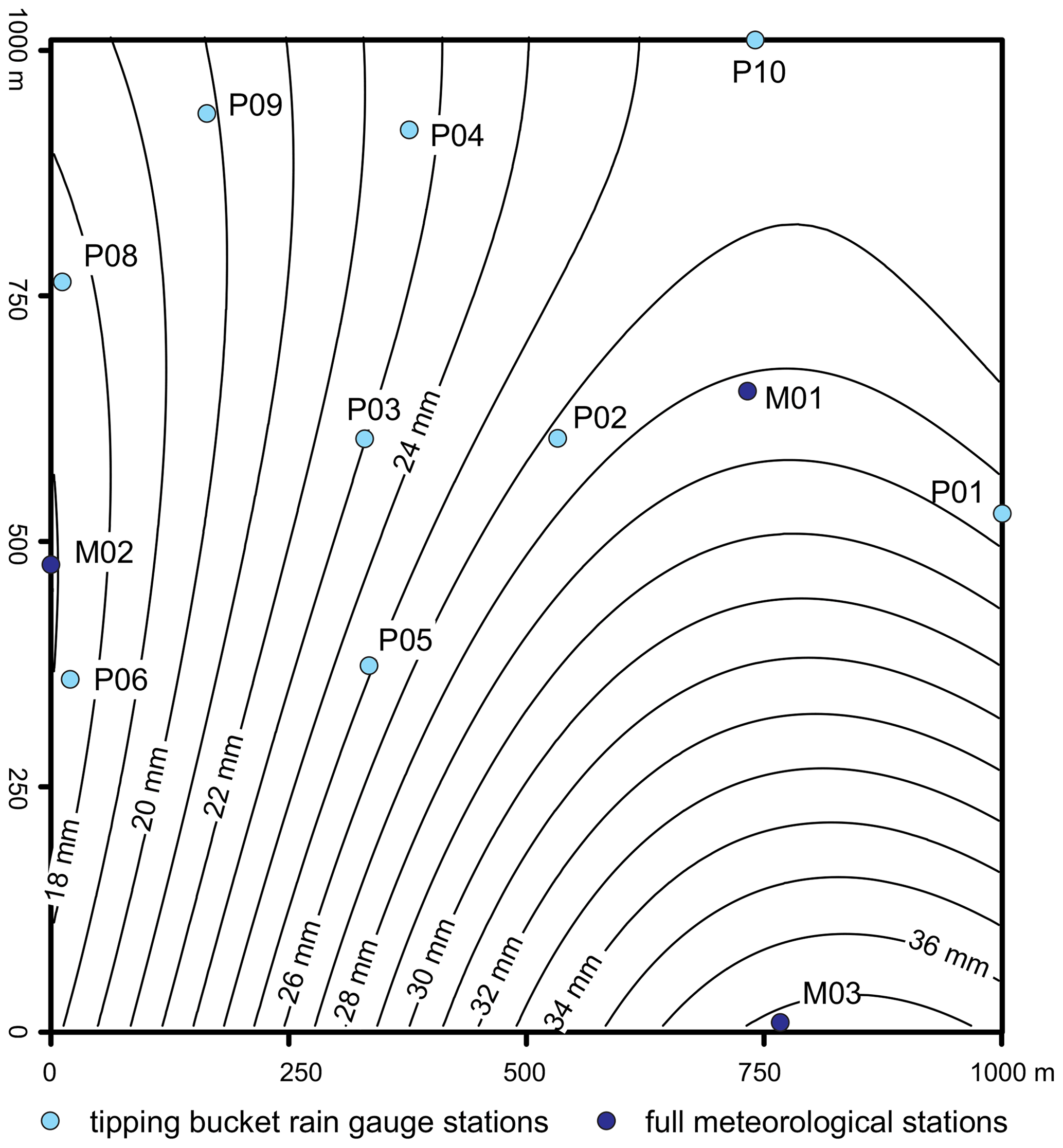
Figure 8Geostatistically interpolated rain depth (mm) of an erosive event with a substantial rainfall gradient (event 116, 26 August 1996); average rain depth calculated from the geostatistical interpolation in 10 m×10 m blocks was 23.6 mm and average gradient in rain depth was 15.7 mm km−1. Figure adapted from Fiener and Auerswald (2009).
More generally, the dataset indicated that a comparison of watersheds with different land use or management can only be reasonably done if the variability in soil properties is taken into account. This is even more important for variables with pronounced spatio-temporal dynamics like field-specific soil cover (Fig. 6) or spatial rainfall gradients of large events (Fig. 8). The latter were studied at the test site for four years using 12 rain gauges. These data indicated that 50 % of all erosive events had substantial spatial rainfall gradients. Variation in rain erosivity was up to 255 % and thus much more pronounced than the variation in total rain depth (for details see Fiener and Auerswald, 2009). Even for the rainfall event with the largest erosivity (approximately half of the long-term mean annual erosivity) in the data set, erosivity was zero within a distance of about 500 m (Fischer et al., 2018). By analysing a much larger data set of about 40 000 erosive events in Germany, Fischer et al. (2018) showed that this extreme behaviour of including zero within such a short distance was true for about half of all events but that strong gradients existed also for most of the other events. This emphasized that also for small watersheds, spatial variability in rainfall has to be taken into account.
Watershed studies are indispensable to understand soil erosion as they integrate (i) real agricultural practices, (ii) natural heterogeneity along the flow path, and (iii) realistic field sizes and layouts. However, there is a prominent lack of watershed studies, (1) which observed watersheds small enough to associate runoff and soil delivery with individual land uses, (2) which are considerably smaller than erosive rain cells (<400 ha), (3) which cover many years to account for the variability of rain regarding erosivity and timing, (4) which combine many watersheds to allow comparisons, (5) which obtained topographic, pedological, agricultural and meteorological variation in high spatial and temporal resolution, and (6) which were made available. Here we provide such a dataset.
An 8 year monitoring in 14 watersheds yielded unprecedented high resolution data in time and space. The data may be used for in-depth analyses or in modelling studies to disentangle the complex interactions that result from the simultaneous variation in space and in time, which is most pronounced for crop development but which involves all other parameters as well.
The data were gathered under conditions where field layout and field managements were optimized to reduce soil loss. Under such conditions, the importance of rare events increases and requires long measuring intervals. This was illustrated by the still large uncertainties of mean surface runoff and sediment delivery (mean 95 %-confidence interval of ±75 % and ±95 % in case of surface runoff and sediment delivery, respectively). To gather sufficient events under a variety of conditions, 14 watersheds were monitored over 8 year. Six watersheds were subject to the same field management of integrated farming but differed in the position within the 4-year rotation. Eight watersheds were subject to the same field management of organic farming but again differed in the position within the 7-year rotation and covered grassland.
Overall, the presented data set underlined the importance of long-term monitoring to determine the huge temporal variability of surface runoff and sediment delivery from small watersheds. However, to use the full potential of labour intensive long-term monitoring, it is essential that not only runoff and sediment delivery is monitored. We strongly suggest putting more efforts in monitoring of agroecosystem variables (e.g. soil management, soil properties, soil cover, meteorology etc.) that spatially and temporally vary within watersheds.
All data created in this study are freely available. The soil data (Auerswald et al., 2019b) can be obtained from https://doi.org/10.13140/RG.2.2.14231.83365. The topographic data (Wilken et al., 2019a) can be obtained from https://doi.org/10.13140/RG.2.2.32044.51845. The meteorological data (Wilken et al., 2019b) can be obtained from https://doi.org/10.13140/RG.2.2.34561.10088. The land use and land management data (Auerswald et al., 2019d) can be obtained from https://doi.org/10.13140/RG.2.2.26172.49285. The runoff and soil loss data during natural rain events (Fiener et al., 2019) can be obtained from https://doi.org/10.13140/RG.2.2.30786.22729. The runoff and soil loss data from small plots under simulated rainfall (Auerswald et al., 2019c) can be obtained from https://doi.org/10.13140/RG.2.2.27430.78401.
This paper represents a result of collegial teamwork. PF and KA designed the data analysis and prepared the manuscript. All authors conducted the literature research. All authors read and approved the final manuscript.
The authors declare that they have no conflict of interest.
This article is part of the special issue “Innovative monitoring techniques and modelling approaches for analysing hydrological processes in small basins”. It is a result of the 17th Biennial Conference ERB 2018, Darmstadt, Germany, 11–14 September 2018.
The scientific activities of the research network Forschungsverbund Agrarökosysteme München (FAM) were financially supported by the German Federal Ministry of Education and Research (BMBF 0339370). Overhead costs of the research station of Scheyern were funded by the Bavarian State Ministry for Science, Research and Arts. This research, which is a summary of nearly a decade of intensive field monitoring, would have not be possible without the unresting efforts of so many colleagues, technicians, and students. Outstanding contributions were made by Max Kainz, Georg Gerl and Stephan Weigand. The efforts of all collaborators are gratefully acknowledged. This study was also supported by the German Research Foundation (DFG) and the Technical University of Munich (TUM) in the framework of the Open Access Publishing Program.
This research has been supported by the German Federal Ministry of Education and Research (grant no. BMBF 0339370).
This work was supported by the German Research Foundation (DFG) and the Technical University of Munich (TUM) in the framework of the Open Access Publishing Program.
This paper was edited by Britta Schmalz and reviewed by Thomas Hoffmann and one anonymous referee.
Anderson, B. and Potts, D. F.: Suspended sediment and turbidity following road construction and logging in western Montana, Water Resour. Bull., 23, 681–690, 1987.
Auerswald, K.: Infuence of initial moisture and time since tillage on surface structure breakdown and erosion of a loessial soil, Catena Suppl., 24, 93–101, 1993.
Auerswald, K. and Geist, J.: Extent and causes of siltation in a headwater stream bed: catchment soil erosion is less important than internal stream processes, Land Degrad. Dev., 29, 737–748, 2018.
Auerswald, K. and Schimmack, W.: Element-pool balances in soils containing rock fragments, Catena, 40, 279–290, 2000.
Auerswald, K., Kainz, M., Schröder, D., and Martin, W.: Comparison of German and Swiss rainfall simulators – Experimental setup, Zeitschrift für Planzenernährung und Bodenkunde, 155, 1–5, 1992.
Auerswald, K., Albrecht, H., Kainz, M., and Pfadenhauer, J.: Principles of sustainable land-use systems developed and evaluated by the Munich Research Alliance on agro-ecosystems (FAM), Petermanns Geographische Mitteilungen, 144, 16–25, 2000.
Auerswald, K., Kainz, M., Scheinost, A. C., and Sinowski, W.: The Scheyern experimental farm: research methods, the farming system and definition of the framework of site properties and characteristics, in: Ecosystem Approaches to Landscape Management in Central Europe, edited by: Tenhunen, J. D., Lenz, R., and Hantschel, R., Ecological Studies, Berlin, Heidelberg, New York, 2001.
Auerswald, K., Kainz, M., and Fiener, P.: Soil erosion potential of organic versus conventional farming evaluated by USLE modelling of cropping statistics for agricultural districts in Bavaria, Soil Use Manage., 19, 305–311, 2003.
Auerswald, K., Fiener, P., and Dikau, R.: Rates of sheet and rill erosion in Germany – A meta-analysis, Geomorphology, 111, 182–193, 2009.
Auerswald, K., Mayer, F., and Schnyder, H.: Coupling of spatial and temporal pattern of cattle excreta patches on a low intensity pasture, Nutr. Cycl. Agroecosyst., 88, 275–288, 2010.
Auerswald, K., Fiener, P., Martin, W., and Elhaus, D.: Use and misuse of the K factor equation in soil erosion modeling: An alternative equation for determining USLE nomograph soil erodibility values, Catena, 118, 220–225, 2014.
Auerswald, K., Fischer, F., Kistler, M., Treisch, M., Maier, H., and Brandhuber, R.: Behavior of farmers in regard to erosion by water as reflected by their farming practices, Sci. Total Environ., 613–614, 1–9, 2018.
Auerswald, K., Fischer, F. K., Winterrath, T., and Brandhuber, R.: Rain erosivity map for Germany derived from contiguous radar rain data, Hydrol. Earth Syst. Sci., 23, 1819–1832, https://doi.org/10.5194/hess-23-1819-2019, 2019a.
Auerswald, K., Wilken, F., and Fiener, P.: Soil properties at the Scheyern experimental farm covering 14 small adjacent watersheds and their surroundings, ResearchGate, https://doi.org/10.13140/RG.2.2.14231.83365, 2019b.
Auerswald, K., Wilken, F., and Fiener, P.: Runoff and sediment delivery data of 114 rainfall simulation experiments on 57 plots situated in 14 small adjacent watersheds at the Scheyern experimental farm, ResearchGate, https://doi.org/10.13140/RG.2.2.27430.78401, 2019c.
Auerswald, K., Wilken, F., Gerl, G., and Fiener, P.: Land use and land management data from the Scheyern experimental farm covering 14 small adjacent watersheds and their surroundings, ResearchGate, https://doi.org/10.13140/RG.2.2.26172.49285, 2019d.
Baker, J. L. and Johnson, H. P.: The effect of tillage systems on pesticides in runoff from small watersheds, T. Am. Soc. Agric. Eng., 22, 554–559, 1979.
Beasley, R. S.: Intensive site preparation and sediment losses on steep watersheds in the Gulf Coastal Plain, Soil Sci. Soc. Am. J., 43, 412–417, 1979.
Beasley, R. S., Granillo, A. B., and Zillmer, V.: Sediment losses from forest management: mechanical vs. chemical site preparation after clearcutting, J. Environ. Qual., 15, 413–416, 1986.
Becht, M. and Wetzel, K. F.: Dynamik des Feststoffaustrages kleiner Wildbäche in den bayerischen Kalkvoralpen, Göttinger Geographische Abhandlungen, 86, 45–52, 1989.
Bingner, R. L., Murphree, C. E., and Mutchler, C. K.: Comparison of sediment yield models on various watersheds in Mississippi, Am. Soc. Agric. Eng., 32, 529–534, 1989.
Bowie, A. J. and Bolton, G. C.: Variations in runoff and sediment yields on two adjacent watersheds as influenced by hydrologic and physical characteristics, Proc. Mississippi Water Resources Conference, Mississippi State University, 38–55, 1972.
Brooks, E. S., Boll, J., Snyder, A. J., Ostrowski, K. M., Kane, S. L., Wulfhorst, J. D., Van Tassell, L. W., and Mahler, R.: Long-term sediment loading trends in the Paradise Creek watershed, J. Soil Water Conserv., 65, 331–341, 2010.
Carter, C. E. and Parsons, D. A.: Field tests on the Coshocton-type wheel runoff sampler, T. Am. Soc. Agric. Eng., 10, 133–135, 1967.
Casali, J., Gastesi, R., Alvarez-Mozos, J., Santisteban, L. M., Del Vall de Lersundi, J., Giménez, R., Larraąaga, A., Goąi, M., Agirre, U., Campo, M. A., López, J. J., and Donézar, M.: Runoff, erosion, and water quality of agricultural watersheds in central Navarre (Spain), Agr. Water Manage., 95, 1111–1128, 2008.
Cerdan, O., Govers, G., Le Bissonnais, Y., Van Oost, K., Poesen, J., Saby, N., Gobin, A., Vacca, A., Quinton, J., Auerswald, K., Klik, A., Kwaad, F. J. P. M., Raclot, D., Ionita, I., Rejman, J., Rousseva, S., Muxart, T., Roxo, M. J., and Dostal, T.: Rates and spatial variations of soil erosion in Europe: a study based on erosion plot data, Geomorphology, 122, 167–177, 2010.
Chow, T. L., Rees, H. W., and Daigle, J. L.: Effectiveness of terraces/grassed waterway systems for soil and water conservation: A field evaluation, J. Soil Water Conserv., 3, 577–583, 1999.
Coppus, R. and Imeson, A. C.: Extreme events controlling erosion and sediment transport in a semi-arid sub-andean valley, Earth Surf. Proc. Land., 27, 1365–1375, 2002.
Deasy, C., Baxendale, S. A., Heathwaite, A. L., Ridall, G., Hodgkinson, R., and Brazier, R. E.: Advancing understanding of runoff and sediment transfers in agricultural catchments through simultaneous observations across scales, Earth Surf. Proc. Land., 36, 1749–1760, 2011.
Dendy, F. E.: Sediment yield from a Mississippi Delta cotton field, J. Environ. Qual., 10, 482–486, 1981.
Dickinson, W. T. and Scott, A.: Fluvial sedimentation in Southern Ontario, Can. J. Earth Sci., 12, 1813–1819, 1975.
Didone, E. J., Minella, J. P. G., and Evrard, O.: Measuring and modelling soil erosion and sediment yields in a large cultivated catchment under no-till of Southern Brazil, Soil Till. Res., 174, 24–33, 2017.
Diyabalanage, S., Samarakoon, K. K., Adikari, S. B., and Hewawasam, T.: Impact of soil and water conservation measures on soil erosion rate and sediment yields in a tropical watershed in the Central Highlands of Sri Lanka, Appl. Geogr., 79, 103–114, 2017.
Duvert, C., Gratiot, N., Evrard, O., Navratil, O., Nemery, J., Prat, C., and Esteves, M.: Drivers of erosion and suspended sediment transport in three headwater catchments of the Mexican Central Highlands, Geomorphology, 123, 243–256, 2010.
Edwards, W. M., Triplett, G. B., Van Doren, D. M., Owens, L. B., Redmond, C. E., and Dick, W. A.: Tillage studies with a corn-soybean rotation: Hydrology and sediment loss, Soil Sci. Soc. Am. J., 57, 1051–1055, 1993.
Evrard, O., Vandaele, K., Van Wesemael, B., and Bielders, C. L.: A grassed waterway and earthen dams to control muddy floods from a cultivated catchment of the Belgian loess belt, Geomorphology, 100, 419–428, 2008.
Fang, N. F., Wang, L., and Shi, Z. H.: Runoff and soil erosion of field plots in a subtropical mountainous region of China, J. Hydrol., 552, 387–395, 2017.
Fiener, P. and Auerswald, K.: Effectiveness of grassed waterways in reducing runoff and sediment delivery from agricultural watersheds, J. Environ. Qual., 32, 927–936, 2003.
Fiener, P. and Auerswald, K.: Spatial variability of rainfall on a sub-kilometre scale, Earth Surf. Proc. Land., 34, 848–859, 2009.
Fiener, P., Auerswald, K., and Weigand, S.: Managing erosion and water quality in agricultural watersheds by small detention ponds, Agric. Ecosyst. Environ., 110, 132–142, 2005.
Fiener, P., Govers, G., and Van Oost, K.: Evaluation of a dynamic multi-class sediment transport model in a catchment under soil-conservation agriculture, Earth Surf. Proc. Land., 33, 1639–1660, 2008.
Fiener, P., Seibert, S. P., and Auerswald, K.: A compilation and meta-analysis of rainfall simulation data on arable soils, J. Hydrol., 409, 395–406, 2011.
Fiener, P., Auerswald, K., Winter, F., and Disse, M.: Statistical analysis and modelling of surface runoff from arable fields in central Europe, Hydrol. Earth Syst. Sci., 17, 4121–4132, https://doi.org/10.5194/hess-17-4121-2013, 2013.
Fiener, P., Wilken, F., and Auerswald, K.: Runoff and sediment delivery data at the Scheyern experimental farm covering 14 small adjacent watersheds, ResearchGate, https://doi.org/10.13140/RG.2.2.30786.22729, 2019.
Fischer, F., Hauck, J., Brandhuber, R., Weigl, E., Maier, H., and Auerswald, K.: Spatio-temporal variability of erosivity estimated from highly resolved and adjusted radar rain data (RADOLAN), Agric. For. Meteorol., 223, 72–80, 2016.
Fischer, F. K., Winterrath, T., and Auerswald, K.: Temporal- and spatial-scale and positional effects on rain erosivity derived from point-scale and contiguous rain data, Hydrol. Earth Syst. Sci., 22, 6505–6518, https://doi.org/10.5194/hess-22-6505-2018, 2018.
Foster, G. R., Lane, L. J., and Knisel, W. G.: Estimating sediment yield from cultivated fields, Proc. Symposium on watershed management, Am. Soc. Civil. Eng., 151–163, 1980.
Garcia-Ruiz, J. M., Regues, D., Alvera, B., Lana-Renault, N., Serrano-Muela, P., Nadal-Romero, E., Navas, A., Latron, J., Marti-Bono, C., and Arnaez, J.: Flood generation and sediment transport in experimental catchments affected by land use changes in the central Pyrenees, J. Hydrol., 356, 245–260, 2008.
Glendell, M. and Brazier, R. E.: Accelerated export of sediment and carbon from a landscape under intensive agriculture, Sci. Total Environ., 476–477, 643–656, 2014.
Gräler, B., Pebesma, E., and Heuvelink, G.: Spatio-temporal interpolation using gstat, The R Journal, 8, 204–218, 2016.
Grangeon, T., Maniere, L., Foucher, A., Vandromme, R., Cerdan, O., Evrard, O., Pene-Galland, I., and Salvador-Blanes, S.: Hydro-sedimentary dynamics of a drained agricultural headwater catchment: a nested monitoring approach, Vadose Zone J., 16, 1–11, 2017.
Hamlett, J. M., Baker, J. L., and Johnson, H. P.: Channel morphology changes and sediment yield for a small agricultural watershed in Iowa, T. Am. Soc. Agric. Eng., 26, 1390–1396, 1983.
Hasholt, B.: Influence of erosion on the transport of suspended sediment and phosphorus, IAHS Publications, 203, 329–338, 1992.
Hasholt, B. and Styczen, M.: Measurement of sediment transport components in a drainage basin and comparison with sediment delivery computed by a soil erosion model, IAHS Publications, 217, 147–159, 1993.
Inoubli, N., Raclot, D., Moussa, R., Habaieb, H., and Le Bissonnais, Y.: Soil cracking effects on hydrological and erosive processes: a study case in Mediterranean cultivated vertisols, Hydrol. Process., 30, 4154–4167, 2016.
Kaemmerer, A.: Raum-Zeit-Variabilität von Aggregatstabilität und Bodenrauhigkeit, Shaker, Aachen, 2000.
Kainz, M.: Runoff, erosion and sugar beet yields in conventional and mulched cultivation. Results of the 1988 experiment, Soil Technol. Ser., 1, 103–114, 1989.
Kainz, M., Auerswald, K., and Vöhringer, R.: Comparison of German and Swiss rainfall simulators – Utility, labour demands and costs, Zeitschrift für Pflanzenernährung und Bodenkunde, 155, 7–11, 1992.
Kainz, M., Gerl, G., and Auerswald, K.: Verminderung der Boden- und Gewässerbelastung im Kartoffelanbau des ökologischen Landbaus, Mitteilungen der Deutschen Bodenkundlichen Gesellschaft, 85, 1307–1310, 1997.
Khanbilvardi, R. M. and Rogowski, A. S.: Quantitative evaluation of sediment delivery ratios, Water Resour. Bull., 20, 865–874, 1984.
Kimes, S. C. and Baker, J. L.: Sediment transport from field to stream: particle size and yield, Am. Soc. Agric. Eng., 79-2529, 1–36, 1979.
Lochbihler, K., Lenderink, G., and Siebesma, A. P.: The spatial extent of rainfall events and its relation to precipitation scaling, Geophys. Res. Lett., 44, 8629–8636, 2017.
Martinez-Casasnovas, J. A., Ramos, M. C., and Ribes-Dasi, M.: Soil erosion caused by extreme rainfall events: mapping and quantification in agricultural plots from very detailed digital elevation models, Geoderma, 105, 125–140, 2002.
McDowell, L. L., Willis, G. H., and Murphree, C. E.: Plant nutrient yields in runoff from a Mississippi delta watershed, T. Am. Soc. Agric. Eng., 27, 1059–1066, 1984.
Mielke, L. N.: Performance of water and sediment control basins in northeastern Nebraska, J. Soil Water Conserv., 40, 524–528, 1985.
Mildner, W. F. and Boyce, R. C.: Monthly variations between soil loss and sediment yield, Am. Soc. Agric. Eng., 79-2528, 1–13, 1979.
Minella, J. P. G., Merten, G. H., Barros, C. A. P., Ramon, R., Schlesner, A., Clarke, R. T., Moro, M., and Dalbianco, L.: Long-term sediment yield from a small catchment in southern Brazil affected by land use and soil management changes, Hydrol. Process., 32, 200–211, 2018.
Monke, E. J., Nelson, D. W., and Beasley, D. B.: Sediment and nutrient movement from the Black Creek Watershed, Am. Soc. Agric. Eng., 79-2048, 1–25, 1979.
Montanarella, L., Pennock, D. J., McKenzie, N., Badraoui, M., Chude, V., Baptista, I., Mamo, T., Yemefack, M., Singh Aulakh, M., Yagi, K., Young Hong, S., Vijarnsorn, P., Zhang, G.-L., Arrouays, D., Black, H., Krasilnikov, P., Sobocká, J., Alegre, J., Henriquez, C. R., de Lourdes Mendonça-Santos, M., Taboada, M., Espinosa-Victoria, D., AlShankiti, A., AlaviPanah, S. K., Elsheikh, E. A. E. M., Hempel, J., Camps Arbestain, M., Nachtergaele, F., and Vargas, R.: World's soils are under threat, SOIL, 2, 79–82, https://doi.org/10.5194/soil-2-79-2016, 2016.
Morgan, R. P. C., Quinton, J. N., Smith, R. E., Govers, G., Poesen, J. W. A., Auerswald, K., Chisci, G., Torri, D., and Styczen, M. E.: The European soil erosion model (EUROSEM): A dynamic approach for predicting sediment transport from fields and small catchments, Earth Surf. Proc. Land., 23, 527–544, 1998.
Murphree, C. E. and Mutchler, C. K.: Sediment yield from a flatland watershed, T. Am. Soc. Agric. Eng., 24, 966–969, 1981.
Murphree, C. E., Mutchler, C. K., and McGregor, K. C.: Sediment yield from a 259-ha flatlands watershed, T. Am. Soc. Agric. Eng., 28, 1120–1123, 1985.
Mutchler, C. K. and Bowie, A. J.: Effect of land use on sediment delivery ratios, 3rd Federal Interagency Sediment Conference Proceedings, Water Resouces Council, Washington D.C., USA, 1.11–11.21, 1979.
Nearing, M. A., Govers, G., and Norton, D. L.: Variability in soil erosion data from replicated plots, Soil Sci. Soc. Am. J., 63, 1829–1835, 1999.
Nunes, J. P., Bernard-Jannin, L., Blanco, M. L. R., Santos, J. M., Coelho, C. D. A., and Keizer, J. J.: Hydrological and erosion processes in terraced fields: observations from a humid Mediterranean region in northern Portugal, Land Degrad. Dev., 29, 596–606, 2016.
Onstad, C. A., Piest, R., and Saxton, K.: Watershed erosion model validation for Southwest Iowa, in: 3rd Federal Interagency Sediment Conference Proceedings, Water Resouces Council, Washington D.C., USA, 1976.
Pieri, L., Ventura, F., Vignudelli, M., Hanuskova, M., and Bittelli, M.: Rainfall, streamflow and sediment relationship in a hilly semi-agricultural catchment in Northern Italy, Italian Journal of Agrometeorology-Rivista Italiana Di Agrometeorologia, 19, 29–42, 2014.
Pimentel, D.: Soil erosion: A food and environmental threat, Environ. Dev. Sustain., 8, 119–137, 2006.
Pimentel, D. and Burgess, M.: Soil erosion threatens food production, Agriculture, 3, 443–463, 2013.
Porto, P., Walling, D. E., and Callegari, G.: Investigating the effects of afforestation on soil erosion and sediment mobilisation in two small catchments in Southern Italy, Catena, 79, 181–188, 2009.
Ramos, T. B., Goncalves, M. C., Branco, M. A., Brito, D., Rodrigues, S., Sanchez-Perez, J. M., Sauvage, S., Prazeres, A., Martins, J. C., Fernandes, M. L., and Pires, F. P.: Sediment and nutrient dynamics during storm events in the Enxoe temporary river, southern Portugal, Catena, 127, 177–190, 2015.
R-Core-Team: R: A language and environment for statistical computing. R Foundation for Statistical Computing, Vienna, Austria, 2018.
Ribolzi, O., Evrard, O., Huon, S., De Rouw, A., Silvera, N., Latsachack, K. O., Soulileuth, B., Lefevre, I., Pierret, A., Lacombe, G., Sengtaheuanghoung, O., and Valentin, C.: From shifting cultivation to teak plantation: effect on overland flow and sediment yield in a montane tropical catchment, Sci. Rep., 7, 3987, 2017.
Sachs, L.: Applied Statistics. A Handbook of Techniques, New York, Heidelberg, Berlin,1984.
Scheinost, A. C., Sinowski, W., and Auerswald, K.: Regionalization of soil water retention curves in a highly variable soilscape, I. Developing a new pedotransfer function, Geoderma, 78, 129–143, 1997.
Schilling, K. E., Isenhart, T. M., Palmer, J. A., Wolter, C. F., and Spooner, J.: Impacts of land-cover change on suspended transport in two agricultural watersheds, J. Am. Water Resour. As., 47, 672–686, 2011.
Schnyder, H., Locher, F., and Auerswald, K.: Nutrient redistribution by grazing cattle drives patterns of topsoil N and P stocks in a low-input pasture ecosystem, Nutr. Cycl. Agroecosyst., 88, 183–195, 2010.
Schüller, H.: Die CAL-Methode, eine neue Methode zur Bestimmung des pflanzenverfügbaren Phosphats in Böden, Zeitschrift für Planzenernährung und Bodenkunde, 123, 48–63, 1969.
Schwertmann, U., Vogl, W., and Kainz, M.: Bodenerosion durch Wasser – Vorhersage des Abtrags und Bewertung von Gegenmaßnahmen, Ulmer Verlag, Stuttgart, 1987.
Sheridan, J. M., Booram Jr, C. V., and Asmussen, L. E.: Sediment-delivery ratios for a small coastal plain agricultural watershed, T. Am. Soc. Agric. Eng., 25, 610–615, 1982.
Sherriff, S. C., Rowan, J. S., Melland, A. R., Jordan, P., Fenton, O., and Huallacháin, D.: Investigating suspended sediment dynamics in contrasting agricultural catchments using ex situ turbidity-based suspended sediment monitoring, Hydrol. Earth Syst. Sci., 19, 3349–3363, https://doi.org/10.5194/hess-19-3349-2015, 2015.
Simanton, J. R. and Osborn, H. B.: Runoff estimates for thunderstorm rainfall on small rangeland watersheds, Hydrology and Water Resources in Arizona and the Southwest, 13, 9–15, 1983.
Simanton, J. R. and Renard, K. G.: Seasonal change in infiltration and erosion from USLE plots in Southeastern Arizona, Hydrology and Water Resources in Arizona and the Southwest, 12, 37–46, 1982.
Simanton, J. R., Osborn, H. B., and Renard, K. G.: Application of the USLE to southwest rangelands, Hydrology and Water Resources in Arizona and the Southwest, 10, 213–220, 1980.
Sinowski, W. and Auerswald, K.: Using relief parameters in a discriminant analysis to stratify geological areas with different spatial variability of soil properties, Geoderma, 89, 113–128, 1999.
Sinowski, W., Scheinost, A. C., and Auerswald, K.: Regionalization of soil water retention curves in a highly variable soilscape, II. Comparison of regionalization procedures using a pedotransfer function, Geoderma, 78, 145–159, 1997.
Sith, R., Yamamoto, T., Watanabe, A., Nakamura, T., and Nadaoka, K.: Analysis of red soil sediment yield in a small agricultural watershed in Ishigaki Island, Japan, using long-term and high resolution monitoring data, Environ. Process., 4, 333–354, 2017.
Smets, T., Poesen, J., and Bochet, E.: Impact of plot length on the effectiveness of different soil-surface covers in reducing runoff and soil loss by water, Prog. Phys. Geogr., 32, 654–677, 2009.
Sran, D. S., Kukal, S. S., and Singh, M. J.: Run-off and sediment yield in relation to differential gully-plugging schemes in micro-catchments of Shiwaliks in the lower Himalayas, Archives of Agronomy and Soil Science, 58, 1317-1327, 2012.
Starks, P. J., Steiner, J. L., Moriasi, D. N., Guzman, J. A., Garbrecht, J. D., Allen, P. B., and Naney, J. W.: Upper Washita River experimental watersheds: Nutrient water quality data, J. Environ. Qual., 43, 1280–1297, 2014.
Steegen, A., Govers, G., Nachtergaele, J., Takken, I., Beuselinck, L., and Poesen, J.: Sediment export by water from an agricultural catchment in the loam belt of central Belgium, Geomorphology, 33, 25–36, 2000.
Stott, T. A., Ferguson, R. I., Johnson, R. C., and Newson, M. D.: Sediment budgets in forested and unforested basins in upland Scotland, in: IAHS Publication, 159, 57–68, 1986.
Valentin, C., Agus, F., Alamban, R., Boosaner, A., Bricquet, J. P., Chaplot, V., de Guzman, T., de Rouw, A., Janeau, J. L., Orange, D., Phachomphonh, K., Do Duy, P., Podwojewski, P., Ribolzi, O., Silvera, N., Subagyono, K., Thiébaux, J. P., Tran Duc, T., and Vadari, T.: Runoff and sediment losses from 27 upland catchments in southeast Asia: Impact of rapid land use changes and conservation practices, Agric. Ecosyst. Environ., 128, 225–238, 2008.
Van Oost, K., Govers, G., Cerdan, O., Thauré, D., Van Rompaey, A., Steegen, A., Nachtergaele, J., Takken, I., and Poesen, J.: Spatially distributed data for erosion model calibration and validaton: The Ganspoel and Kinderveld datasets, Catena, 61, 105–121, 2005.
Vongvixay, A., Grimaldi, C., Dupas, R., Fovet, O., Birgand, F., Gilliet, N., and Gascuel-Odoux, C.: Contrasting suspended sediment export in two small agricultural catchments: Cross-influence of hydrological behaviour and landscape degradation or stream bank management, Land Degrad. Dev., 29, 1385–1396, 2018.
Walling, D. E. and Amos, C. M.: Source, storage and mobilisation of fine sediment in a chalk stream system, Hydrol. Process., 13, 323–340, 1999.
Walling, D. E., Collins, A. L., Sichingabula, H. M., and Leeks, G. J. L.: Integrated assessment of catchment suspended sediment budgets: A Zambian example, Land Degrad. Dev., 12, 387–415, 2001.
Warren, S. D., Hohmann, M. G., Auerswald, K., and Mitasova, H.: An evaluation of methods to determine slope using digital elevation data, Catena, 58, 215–233, 2004.
Wilken, F., Fiener, P., and Auerswald, K.: Topography at the Scheyern experimental farm covering 14 small adjacent watersheds and their surroundings, ResearchGate, https://doi.org/10.13140/RG.2.2.32044.51845, 2019a.
Wilken, F., Fiener, P., and Auerswald, K.: Meteorological data at the Scheyern experimental farm covering 14 small adjacent watersheds and their surroundings, ResearchGate, https://doi.org/10.13140/RG.2.2.34561.10088, 2019b.
Wischmeier, W. H.: Relation of field-plot runoff to management and physical factors, Soil Sci. Soc. Am. Proc., 30, 272–277, 1966.
Wischmeier, W. H. and Smith, D. D.: A universal soil-loss equation to guide conservation farm planning, Trans. 7th Int. Congr. Soil Sci., 418–425, 1960.
Wischmeier, W. H. and Smith, D. D.: Predicting rainfall erosion losses – a guide to conservation planning, U.S. Gov. Print Office, Washington, D.C., 1978.
Wischmeier, W. H., Johnson, C. B., and Cross, B. V.: A soil erodibility nomograph for farmland and construction sites, J. Soil Water Conserv., 26, 189–193, 1971.
WRB: World Reference Base for Soil Resources 2014, update 2015 International soil classification system for naming soils and creating legends for soil maps, FAO, Rome, 2015.
Zhang, Z. Y., Sheng, L. T., Yang, J., Chen, X. A., Kong, L. L., and Wagan, B.: Effects of land use and slope gradient on soil erosion in a red soil hilly watershed of southern China, Sustainability, 7, 14309–14325, 2015.
Zuazo, V. H. D., Martinez, J. R. F., Tejero, I. G., Pleguezuelo, C. R. R., Raya, A. M., and Tavira, S. C.: Runoff and sediment yield from a small watershed in southeastern Spain (Lanjaron): Implications for water quality, Hydrolog. Sci. J., 57, 1610–1625, 2012.