 | 19 Jul 2018
Probabilistic short term wind power forecasts using deep neural networks with discrete target classes
Frank Sehnke
Kay Ohnmeiß
Leon Schröder
Constantin Junk
Anton Kaifel
Usually, neural networks trained on historical feed-in time series of wind turbines deterministically predict power output over the next hours to days. Here, the training goal is to minimise a scalar cost function, often the root mean square error (RMSE) between network output and target values. Yet similar to the analog ensemble (AnEn) method, the training algorithm can also be adapted to analyse the uncertainty of the power output from the spread of possible targets found in the historical data for a certain meteorological situation. In this study, the uncertainty estimate is achieved by discretising the continuous time series of power targets into several bins (classes). For each forecast horizon, a neural network then predicts the probability of power output falling into each of the bins, resulting in an empirical probability distribution. Similiar to the AnEn method, the proposed method avoids the use of costly numerical weather prediction (NWP) ensemble runs, although a selection of several deterministic NWP forecasts as input is helpful. Using state-of-the-art deep learning technology, we applied our method to a large region and a single wind farm. MAE scores of the 50-percentile were on par with or better than comparable deterministic forecasts. The corresponding Continuous Ranked Probability Score (CRPS) was even lower. Future work will investigate the overdispersiveness sometimes observed, and extend the method to solar power forecasts.


The production of wind power predictions with artificial neural networks (ANN) and other machine learning (ML) methods has become commonplace in today's energy meteorology services. Recent advances in the field lead to the development of Deep Neural Networks (Schmidhuber, 2015) and associated software packages to enable their training on graphics cards processors (GPUs). Utilising GPUs leads to a much higher computation speed per unit of power and money.
While this is a very efficient and effective way to generate deterministic forecasts, the growing demand for detailed error information in the forecast poses new challenges. One popular option for providing probability distribution functions (PDFs) instead of point forecasts is to use the calibrated output from ensemble forecast models (Toth and Kalnay, 1993). However, this is somewhat at odds with the ML approaches, since these data driven methods rely on measured target values to train the models. In this case the measured target values are historical wind power time series. Therefore there is only one common “truth” for all ensemble members. To our knowledge, how to pass on the probabilistic information from the ensemble to an ANN is an unsolved problem.
There are alternatives, however: In the so-called Analog Ensemble (AnEn) method (Delle Monache et al., 2011; Junk et al., 2015; Van den Dool, 1989), a historical record of forecasts from one deterministic NWP model is searched for similarities to the current forecast. A forecast PDF is then constructed from the spread of the target values corresponding to those historical forecast situations. This is already very similar to what a ANN training algorithm does: It looks for patterns in the historical input NWP forecasts that correspond to the current situation, and produces a power forecast by weighting the most likely target values in the historical situations. The only element that is missing is to give the ANN a means of expressing its internally constructed PDF for the forecast.
An empirical PDF can be implemented by splitting the continuous target values into several classes representing probabilities. This is described in Sect. 2, together with our network setup and the data used. In Sect. 3 we present the most important findings before wrapping up in Sect. 4.
We demonstrate the new method on two different historical wind power data sets (Table 1): One stems from a wind farm located in northern Germany. The other set is the sum of all wind farms feeding into the German grid, as calculated by the German energy exchange (EEX). These two datasets comprise our target time series.
The system uses different relevant fields from the GFS-4, IFS and HIRLAM NWP models as predictors. In addition, live data from the wind farm as well as aggregated wind power from EEX are ingested (Table 2). Generally, at least one year of data should be available for properly training the model. Note that by supplying the training algorithm with data from three different NWP models, we are actually combining the AnEn methodology with a heterogeneous 3-member-ensemble, providing additional variability information to the DNN. In theory, this could be extended to the 20+ members of a regular ensemble model, but in practice the sheer size of the resulting DNN input vector would prevent this, among other issues, the discussion of which is beyond the scope of this paper.
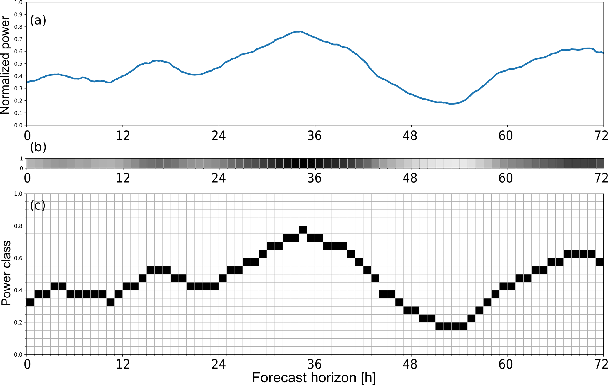
Figure 1(a) Targets (= observations) belonging to one forecast run. (b) Conventional encoding: one continuously valued out-put neuron per forecast horizon. (c) Probabilistic encoding: 20 output neurons per forecast horizon. The one representing the correct power class is set to unity, the others to zero.
We aim to produce a forecast every hour. Therefore for each hour where all input data are available, an input vector is compiled from the NWP forecasts and the other data shown in Table 2. Together with the corresponding power production data as target values, this is called a “pattern”. The total number of patterns available for each setup can be found in Table 1. These numbers include the test set.
From each pattern data set, a test set is separated, which is only utilised for evaluation of the fully trained models. The rest of the data is used by the training framework described below.
In deterministic prediction schemes using ANN, the targets are simply historical wind power observations for each forecast horizon, normalised to installed capacity. In our method, the targets are instead discretised into 20 bins, leading to a 2-D target matrix for each training pattern (Fig. 1c). While this increases the target vector size and the last neuron layer's weight matrix size by an order of magnitude, training times have not been observed to increase considerably. Since we use our highly specialized Learn-O-Matic framework for training the deep neural networks automatically and efficiently (Sehnke et al., 2012), flexibility regarding the output layer error function is somewhat limited. It turned out that training DNN with the new target encoding worked well with the common quadratic error function. Mathematically more rigorous experiments using other, more flexible ML frameworks with e.g. cross entropy error function and softmax output activation function are planned for the future.
Table 1Historical wind power data used for the experiments. For the wind farm, 12 random months were held back as test data. The time ranges include start and end years, but contain periods of missing data. One training pattern per hour was generated for these experiments.
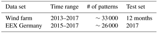
Table 2Input data for the DNN models, the setup of which was derived from previous experiments with deterministic forecasts. We use several wind power relevant fields from each NWP model, at nodes spread around the region of interest. Pi means a “physical” power forecast without corrections, derived by interpolating the respective NWP model to the wind farm location and passing it through the plant's power curve. Pw is a capacity weighted sum of the same quantity over Germany.
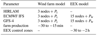

Figure 2Example forecasts with raw probabilistic output. The shading indicates probability per normalised power bin. The median of the distribution and a deterministic reference run are also shown.
Experiments have shown that DNN with two hidden layers are appropriate to find a good solution for this kind of problem. We apply meta optimization to find layer dimensions and the weight decay parameter, as well as automatic feature selection to remove redundancies from the input vector (Sehnke et al., 2012). The DNN are then trained on several NVIDIA GPUs using the well-tried RPROP algorithm (Riedmiller and Braun, 1993).
For each forecast horizon, the trained system produces an empirical power distribution learned from the variety of similar situations in the training data set.
Figure 2 shows examples of such distributions for different situations in the EEX test data set. The data shown are already filtered for outliers and normalized, such that the integral over the histogram at each forecast horizon equals unity. As mentioned above, this is necessary due to the use of a regular RMSE output layer. Interestingly though, the sum of all output neurons at each forecast horizon usually turned out to fall between 0.9 and 1.1, even before normalisation. For all practical purposes we henceforth treat the resulting normalized histograms as PDFs.
As can be seen, the distribution median is systematically lower than the deterministic forecast. The latter minimizes the quadratic difference to the target, and thus rather represents a mean value. Hence, due to the underlying left-skewed distribution of the target values (not shown), the median ends up lower. In addition to the median, the PDFs can be processed into percentiles or other statistical quantities, just like the output from an ensemble forecast model.
A number of validation scores are computed on the test dataset, which, as mentioned above, comprises only historical data that has been held back from training. To compare the deterministic forecast with the PDFs, we calculate the continuous ranked probability score (CRPS), which is equivalent to the mean absolute error (MAE) in the case of a deterministic forecast (Hersbach, 2000). As can be gathered from Fig. 3a, the distribution median performs exactly as well as the deterministic forecast in the Germany case, whereas Fig. 3b shows that it performs even better than the deterministic forecast at higher lead times. The reason for this behaviour is, that as the information in the input NWP forecasts decreases with the forecast horizon, the RMSE-optimizing deterministic forecast tends to the mean, i.e. it almost never outputs values near the minimum (0) or maximum (1) of the normalized power. For the Germany forecast, the target values almost never touch 0 or 1, hence this case does not occur. On the other hand, the deterministic forecast always yields slightly lower RMS errors than the distribution median (not shown), due to the inherent bias of the median.
In both cases however, it can clearly be seen that the CRPS of the PDF forecasts is significantly lower than the MAE. This shows that the PDF does in fact contain additional information about the targets, which may be exploited by the forecast's users. The PDF forecasts still leave room for improvement, as shown in Fig. 4. Here, we note that the distribution is quite overdispersive at short lead times. This effect is currently being investigated, but one reason could be the loss of information due to the discretization of the targets. At longer lead times, this issue vanishes as other error sources become more important than the discretization error. Also, the lowermost percentiles seem to be systematically low, such that too few observed targets fall below them. This may be due to the unequal distribution of target classes: Due to the underlying power distribution, the lowest power classes contain the most values, which may lead to error imbalances during training.
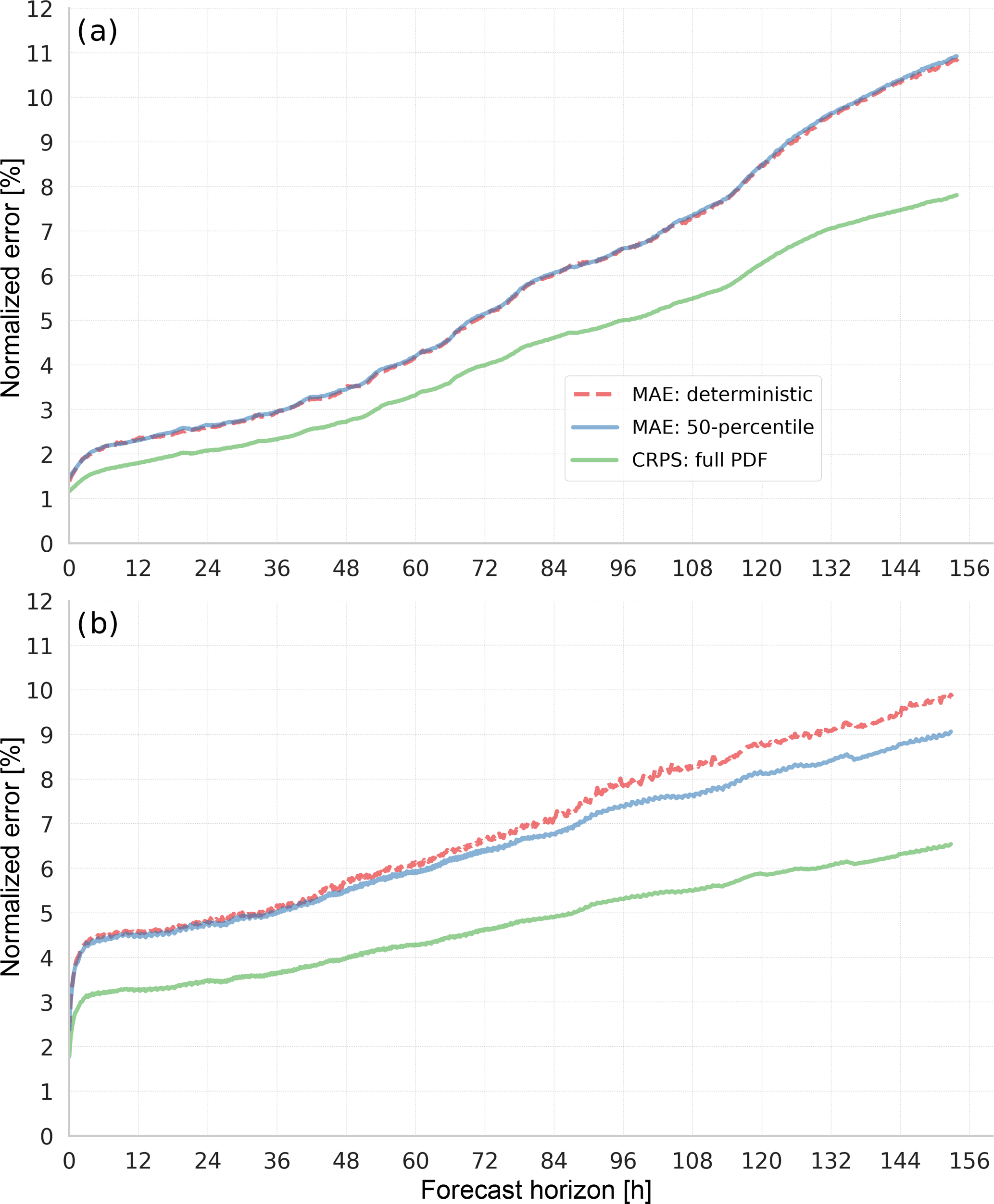
Figure 3Comparing CRPS scores of the full distribution with the equivalent MAE of deterministic forecasts and the distribution median (50-percentile) shows the additional information from the probabilistic output. (a) Germany, EEX energy trading data. (b) Single wind farm.
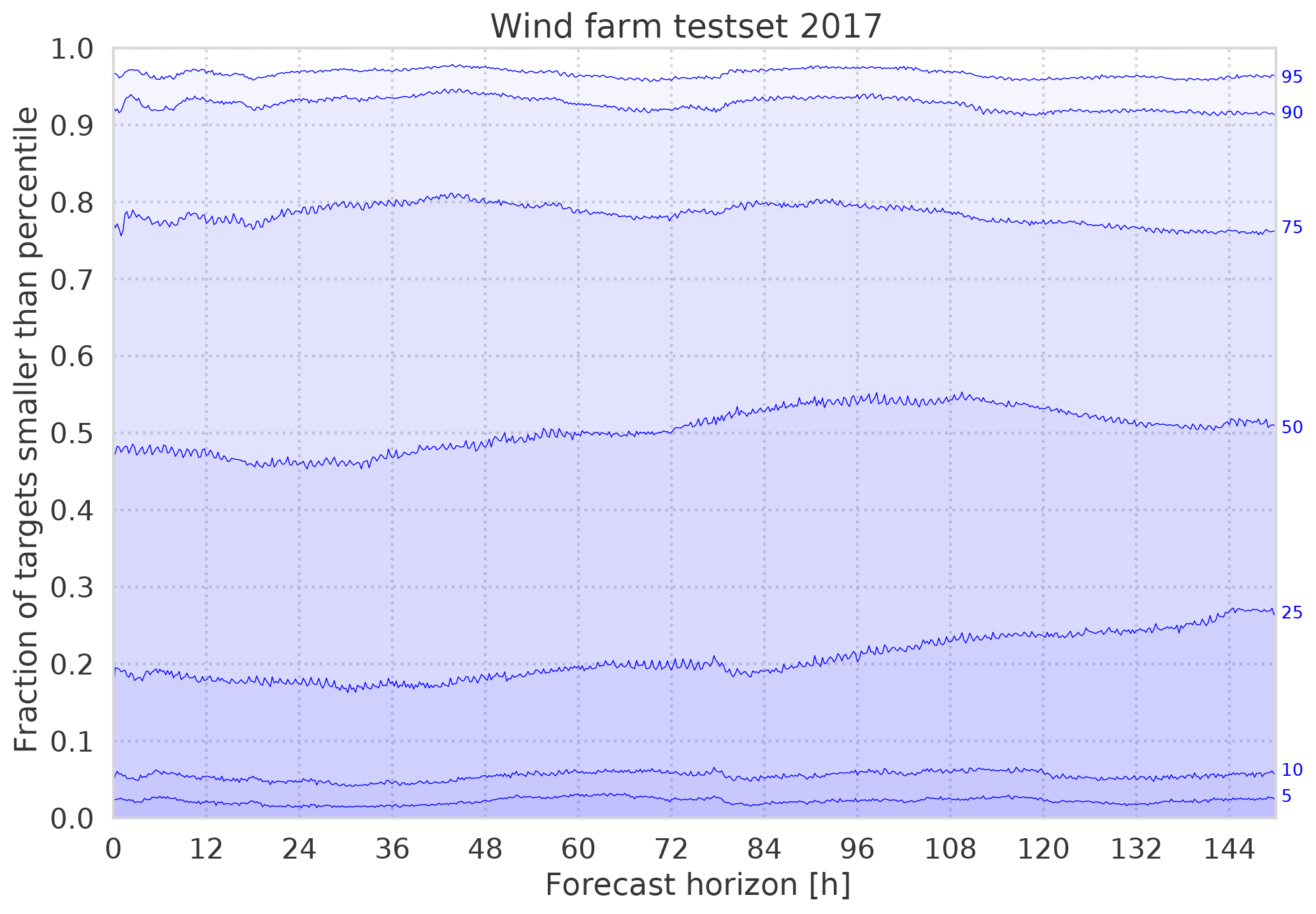
Figure 4To validate the resulting error distributions over the forecast horizon, the fraction of observed test set target values below certain percentiles (blue labels on the right) are plotted. For example, at 48 h lead time, only about 5 % of the test data fall below the 10-percentile, which means that small power output values are generally underrepresented in the class histograms.
A prototype method to produce PDF wind power forecasts using only recent wind power measurements as well as deterministic historical forecasts from one or more NWP models was successfully demonstrated. It is conceptually similar to the AnEn method but based on Deep Neural Networks. It can be applied to wind power forecasts at all aggregation levels.
By means of this method, it is possible to deliver more detailed probability information about short term wind power to decision makers without the need for a comprehensive NWP model ensemble and the large computation time, storage and bandwidth requirements that come with it. However, the method depends on the availability and quality of historical data, hence it may not be applicable everywhere from the start.
From the discrete PDFs we can calculate percentiles and other statistical parameters. It has been found that when MAE is used as a quality criterion, the distribution median performs as well or better than a conventional, deterministic forecast using a DNN trained on the same data. The CRPS calculated on the PDF forecasts outperforms the deterministic forecast's MAE by a large margin.
Future work may include better tuning of the output distributions, adaptation to solar PV forecasts and operational implementation.
Data can be provided upon request, but are partially subject to non-disclosure agreements.
MF designed and carried out the experiments, using software contributions from KO. FS and LS provided input to DNN setup and training procedure. CJ delivered data and input regarding the AnEn method. AK oversaw the project. MF prepared the manuscript with input from all co-authors.
The authors declare that they have no conflict of interest.
This article is part of the special issue “European Geosciences Union General Assembly 2018, EGU Division Energy, Resources & Environment (ERE)”. It is a result of the EGU General Assembly 2018, Vienna, Austria, 8–13 April 2018.
This work was supported through grants 01DN15022 (BMBF) and 0325722A (BMWi)
by the Government of Germany.
Edited by: Michael Kühn
Reviewed by: Johannes Schmidt and one anonymous referee
Delle Monache, L., Nipen, T., Liu, Y., Roux, G., and Stull, R.: Kalman filter and analog schemes to postprocess numerical weather predictions, Mon. Weather Rev., 139, 3554–3570, 2011. a
Hersbach, H.: Decomposition of the continuous ranked probability score for ensemble prediction systems, Weather Forecast., 15, 559–570, 2000. a
Junk, C., Delle Monache, L., Alessandrini, S., Cervone, G., and von Bremen, L.: Predictor-weighting strategies for probabilistic wind power forecasting with an analog ensemble, Meteorol. Z., 24, 361–379, 2015. a
Riedmiller, M. and Braun, H.: A direct adaptive method for faster backpropagation learning: The RPROP algorithm, in: Proc. of IEEE International Conference on Neural Networks, IEEE, 28 March–1 April 1993, San Francisco, CA, USA, 586–591, https://doi.org/10.1109/ICNN.1993.298623, 1993. a
Schmidhuber, J.: Deep learning in neural networks: An overview, Neural networks, 61, 85–117, 2015. a
Sehnke, F., Felder, M., and Kaifel, A.: Learn-O-Matic – Fully automated machine learning, Tech. rep., ZSW Baden-Württemberg, Stuttgart, Germany, 2012. a, b
Toth, Z. and Kalnay, E.: Ensemble forecasting at NMC: The generation of perturbations, B. Am. Meteorol. Soc., 74, 2317–2330, 1993. a
Van den Dool, H.: A new look at weather forecasting through analogues, Mon. Weather Rev., 117, 2230–2247, 1989. a